Return to computing page for the first course APMA0330
Return to computing page for the second course APMA0340
Return to computing page for the fourth course APMA0360
Return to Mathematica tutorial for the first course APMA0330
Return to Mathematica tutorial for the second course APMA0340
Return to Mathematica tutorial for the fourth course APMA0360
Return to the main page for the first course APMA0330
Return to the main page for the second course APMA0340
Return to the main page for the fourth course APMA0330
Return to Part V of the course APMA0340
Introduction to Linear Algebra with Mathematica
This section is about a classical integral transformation, known as the
Fourier
transformation. Since the Fourier transform is expressed through an indefinite integral, its numerical evaluation is an ill-posed problem. It is a custom to use the Cauchy principle value regularization for its definition, as well as for its inverse. It gives the spectral decomposition of the derivative operator \( {\bf j}\,\texttt{D} , \) where \( \texttt{D} = {\text d}/{\text d}x \) and j is the unit vector in the positive vertical direction on the complex plane ℂ. It is a wide area and books are written for this subject. Therefore, we are forced to include only basic results that we cannot avoid when dealing with differential equations.
There are several common conventions for defining the Fourier transform of an integrable
complex-valued function f : ℝ → ℂ.
In applications, the function f(x) is usually referred to as a
signal.
Here we will use the following definition, which is most common in
applications. The Fourier transform of the function f is traditionally denoted
by adding a circumflex:
\( \displaystyle {\hat {f}} \) or \( ℱ\left[ f \right] \) or \( f^F . \)
Actually, the Fourier transform measures the frequency content of the signal
f.
The exponential Fourier transform (or spectrum) of the function f is the complex-valued function defined for the real variable ξ defined (if it exists) as an improperRiemann integral
where \( \xi\cdot t = \xi_1 t_1 + \xi_2 t_2 + \cdots + \xi_n t_n \) is
the inner product and j is the unit vector in the positive
vertical direction on the complex plane ℂ so j² =
-1. The prefix V.P. indicates that the improper integral is evaluated
in the Cauchy principal value sense.
The functions f and
\( \displaystyle {\hat {f}} \) often are referred to as a Fourier integral pair or Fourier transform pair.
The Fourier transform is usually defined in some function spaces. The most common spaces are defined below.
Let 𝔏¹(ℝ) denote the space of functions on ℝ that are Lebesgue-integrable on (−∞, ∞) functions with the norm
\[
\| f \| = \| f \|_1 = \int_{-\infty}^{\infty} \left\vert f(t) \right\vert {\text d}t < \infty .
\]
In this space, all functions which are equal almost everywhere are identified.
The space 𝔏∞(ℝ) is the vector space of bounded measurable functions on ℝ, with the sup norm defined by
Theorem 1:
Let f∈𝔏¹(ℝ) be a function which is Lebesgue-integrable on ℝ. Then its Fourier transform
ξ → fF(ξ) of f is a continuous bounded function for all ξ ∈ ℝ. So \( ℱ \) : 𝔏¹(ℝ) → 𝔏∞(ℝ) and \( \| f^{F} \|_{\infty} \le \| f \|_1 . \)
Theorem 2:
Let f ∈ 𝔏¹(ℝ) be an integrable function such that its Fourier transform fF is itself integrable. Then
\[
ℱ^{-1} \left[ f^F \right] = f(x) \qquad \mbox{for almost all }x \in\mathbb{R} .
\]
There are some functions that are not necessarily integrable, but whose square is. Such is the “sine cardinal” function: \( \mbox{sinc}(x) = x^{-1} \sin x . \) It turns out that in physics, square integrable functions are of paramount importance and occur frequently. It is therefore advisable to extend the definition of the Fourier transform to the class of square integrable functions.
Let 𝔏²(ℝ) denote the space of measurable functions defined on ℝ, with complex values (up to equality almost everywhere) which are square integrable, with the norm
\[
\left\langle f , g \right\rangle = \int_{-\infty}^{\infty} \overline{f}(t)\,g(t)\, {\text d}t ,
\]
𝔏²(ℝ) becomes the Hilbert space. The Fourier transform maps 𝔏²(ℝ) → 𝔏²(ℝ) as an (isometric) isomorphism.
A fundamental result due to Riesz and Fischer, which is not obvious at all,shows that 𝔏²(ℝ) is complete.
Note that the inverse Fourier transformation is an ill-posed problem; therefore, its application must be done with care (see Kabanikhin's survey).
In the above definition, the principle value means that the limit is taken over
symmetrical interval
So the standard definition requires that both bounds N and M approach infinity independently of each other.
The Fourier transformation and its inverse are a bounded operations in the space of square
integrable functions denoted by 𝔏² (other common notations are L² or L2). The following equality is known as Parseval's formula:
Plancherel's Theorem:
The Fourier transform is an isometry on 𝔏², that is,
\( \| f \|_{𝔏^2}^2 = \int_{-\infty}^{\infty} | f(x) |^2
{\text d}x = \left( 2\pi \right)^{-1} \int_{-\infty}^{\infty} | \hat{f}(\xi ) |^2 {\text d}\xi
= \left( 2\pi \right)^{-1} \| \hat{f} \|_{𝔏^2}^2 . \) In multidimensional case, we have
Recall that a real-valued function f : ℝ → ℝ is called an absolutely integrable function if it is a function whose absolute value is integrable, meaning that the integral of the absolute value over the whole domain is finite:
\begin{equation} \label{EqT.6}
\| f \|_1 = \int_{-\infty}^{\infty} \left\vert f(x) \right\vert {\text d} x < \infty .
\end{equation}
We abbreviate it as f ∈ 𝔏¹(ℝ).
A square-integrable function, also called a quadratically integrable function or 𝔏²(ℝ) is a real- or complex-valued measurable function for which the integral of the square of the absolute value is finite:
\begin{equation} \label{EqT.7}
\| f \|^2_2 = \int_{-\infty}^{\infty} \left\vert f(x) \right\vert^2 {\text d} x < \infty .
\end{equation}
A function of bounded variation is a real-valued function whose total variation is bounded (finite). This is equivalent to say that the function has on a compact interval finite number of maximum and minimum; a function of finite variation can be represented by the difference of two monotonic functions having discontinuities, but at most countably many. Obviously, a function of bounded variation cannot have an infinite jump. A real-valued function f is said to satisfy the Dirichlet conditions if
f is absolutely integrable.
f is of bounded variation in any given compact interval.
f must have a finite number of discontinuities in any given bounded interval, and the discontinuities cannot be infinite.
A sufficient condition for exitence of the Fourier transform \( \displaystyle {\hat {f}} \) is its absolutely integrability, f ∈ 𝔏¹(ℝ). In this case, \( \displaystyle {\hat {f}} \) is uniformly continuous on ℝ and
The inversion Fourier transformation formula is based on the following
statement.
Lemma: If a function f(x+u) satisfies the Dirichlet conditions in an interval 𝑎 < u < b, then
\[
\lim_{\omega \to \infty} \frac{2}{\pi} \int_a^b f(x+u) \,\frac{\sin\,\omega u}{\omega}\,{\text d} u = \begin{cases}
f(x+0) + f(x-0) , & \ \mbox{ if } a < 0 < b ,
\\
f(x+0) , & \ \mbox{ if } a=0 < b ,
\\
f(x-0) , & \ \mbox{ if } a < 0 = b ,
\\
0 , & \ 0 < a < b \mbox{ or } a < b < 0 .
\end{cases}
\]
The Fourier integral exists not for arbitrary functions, but for functions that approached zero at infinity. Although the exponential Fourier integral may not converge for a particular function f, the following functions
where ξ = u + jv, may exist: the latter for large enough positive v, and the former for large in absolute value negative v. The inverse Fourier transform gives
The statement that f can be reconstructed from
\( \displaystyle {\hat {f}} \)
is known as the Fourier inversion theorem, and was first introduced in Fourier'sAnalytical Theory of Heat.
Example 2:
Suppose a function f(t) and its derivative df/dt are both piecewise continuous functions for all t ≥ 0. If the function f(t) is not integrable, then its Fourier transfom does not exist. However, it may happen that f(t) times an exponentially decay function could be integrable, so the Fourier transform of such product exists. We define an extension
\[
g(t) = \begin{cases}
e^{-ct} f(t) , & \ \mbox{ for } t \ge 0, \\
0, & \ \mbox{ for } t < 0,
\end{cases}
\]
where c is a positive real constant. Then obviously
\( \int_{\mathbb{R}} \left\vert g(t) \right\vert {\text d}t < \infty , \) is convergent so that its Fourier transform exists. According to the Fourier integral theorem
The latter is used in Mathematica under the name FourierTransform.
There is no agreement on what particular definition of Fourier transform to be
used. Of course, theoretical expositions of this topic prefer to use unitary
versions.
Theorem 5:
The Fourier transformation gives the spectral representation of the derivative operator
\( \displaystyle {\bf j}\,\frac{\text d}{{\text d} x} ,
\) that is,
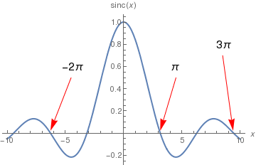
The sinc function sinc(x) is a function that arises frequently in signal processing and
the theory of Fourier transforms. Its inverse Fourier transform is called the
"sampling function" or "filtering function." The full name of the function
is "sine cardinal," but it is commonly referred to by its abbreviation, "sinc."
In Mathematica, sinc function has a default notation: Sinc[x].
The zero crossings of the unnormalized sinc are at non-zero integer multiples
of π, while zero crossings of the normalized sinc occur at non-zero integers.
The function \( \displaystyle y(x) = a\,\mbox{sinc}(a\,x)
= \frac{\sin ax}{x} \) is a bounded solution of the initial value problem for the following second order differential
equation with regular singular point at the origin
Limit[Integrate[(1 + x^2)^(-1) *a*Sinc[a*x], {x, -Infinity,
Infinity}], a -> Infinity]
\[Pi]
The other solution \( \displaystyle \frac{\cos ax}{x} \)
of the differential equation \( x\, y'' + 2\,y' + a^2 x\,y =0 \) is unbounded at x = 0, unlike its sinc function counterpart;
obviously, sinc(0) = 1.
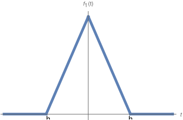
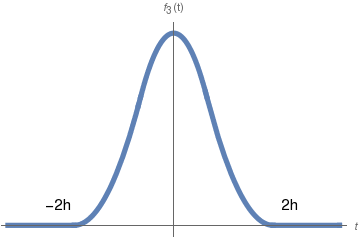
The sinc function is a Forier transform of the tent function
\[
f(x) = \begin{cases}
0, & \ \mbox{ for} \quad x < -w , \\
h \left( 1 - \frac{|x|}{w} \right) , & \ \mbox{ for} \quad |x| < w , \\
0, & \ \mbox{ for} \quad x > w.
\end{cases}
\]
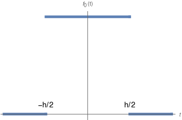
Example 3:
In applications, it is common to approximate functions with piecewise constant
(or step) functions. Although these functions are simple, they are very
important: they are used to approximate other more complicated functions.
A piecewise function is a function that is defined by several subfunctions.
If each piece is a constant function, then the piecewise function is called
Piecewise constant function or Step function. Let us consider one of them:
This step function is commonly referred to as filtering function because the
multiplication by it leads to elimination of the high frequency contributions
to the signal. Therefore, it is also called a low-pass filter.
Its Fourier transform is
We verify the answers with standard Mathematica commands:
f0[x_] = Refine[Piecewise[{{1, -a < x < a}}], a > 0];
Sqrt[2*Pi]*Refine[FourierTransform[f0[x], x, s], a > 0]
(2 Sin[a s])/s
and
Refine[InverseFourierTransform[a*Sinc[a*x], x, t], a > 0]/Sqrt[2*Pi]
1/4 (Sign[a - t] + Sign[a + t])
Note that Mathematica uses the unitary definition for Fourier
transformations and its inverse:
\( \displaystyle f^F (\xi ) = \frac{1}{\sqrt{2\pi}}
\int f(x)\,e^{{\bf j} x\cdot \xi} \,{\text d} x \) and
\( \displaystyle f (x ) = \frac{1}{\sqrt{2\pi}}
\int f^F (\xi )\,e^{-{\bf j} x\cdot \xi} \,{\text d} \xi . \)
Multiplying the Fourier transform \( \hat{f} (\xi ) \)
by the low-pass filter Π(ξ) effectively clips all the high
frequencies (those of frequencies that are > ξ). By taking the inverse
transform of this product, we remove the contribution of the high frequencies
of the signal f(x). Calculations show that
The main property of the Fourier transform is that it gives the spectral
representation of the impulse operator
\( \displaystyle T = {\bf j}\,\frac{\text d}{{\text d}x} . \)
Theorem 8:
If a differentiable function is absolutely integrable, that is
\( f \in 𝔏^1 \left( {\mathbb R}^n \right) , \) and
\( \partial f/\partial x_j \in 𝔏^1 \left( {\mathbb R}^n
\right) , \) then the Fourier transform of the derivative is
So the limit in the right-hand side does not exist because the exponential function \( e^{{\bf j}B\xi} \) has no limit at infinity. Now we find its limit in weak sense. Choosing a probe function
ϕ, we multiply by it and integrate:
To find its value, we connect the end points -K and K on real axis ℝ with semi-circle in complex plane ℂ to make a close loop. Then we apply the residue theorem. Since we have half of a circle, we have only half of the residure:
There are known two spectral representations for the product of the impulse
operator \( \displaystyle \left( {\bf j} \,\frac{\text d}{{\text d}x} \right)^2 = - \frac{{\text d}^2}{{\text d}x^2} . \) They can be derived from the main Fourier formula for either even
function, f(-x) = f(x) or odd function,
f(-x) = -f(x). Correspondingly, we obtain the
cosine Fourier transformation and sine Fourier transformation.
For an integrable on the interval [0, ∞) function f, two
transformations can be defined; one is called cosine Fourier transform:
\[
ℱ_c \left[ f \right] (s) = f^c (s) =
\int_0^{\infty} f(x)\,\cos (sx) \,{\text d}x
\qquad\mbox{and} \qquad f(x) = \frac{2}{\pi} \int_0^{\infty}
ℱ_c \left[ f \right] (s)\,\cos (sx) \,{\text d}s ;
\]
and sine Fourier transform:
\[
ℱ_s \left[ f \right] (s) = f^s (s) =
\int_0^{\infty} f(x)\,\sin (sx) \,{\text d}x
\qquad\mbox{and} \qquad f(x) = \frac{2}{\pi} \int_0^{\infty}
ℱ_s \left[ f \right] (s)\,\sin (sx) \,{\text d}s .
\]
These two transformations provide spectral representations for the second
derivative operator with Dirichlet and Neumann boundary conditions,
respectively. More precisely, we have
Mathematica has two dedicated commands to perform sine and cosine Fourier transforms: FourierSinTransform and FourierCosTransform; however, Mathematica defines its Fourier transforms as:
Talvila, E., Fourier transform inversion using an elementary differential equation and a contour integral, American Mathematical Monthly, 2019, Vol. 126, No. 8, pp.717--727.
Titchmarsh, E.C. Introduction to the Theory of Fourier Integrals, 3rd ed. Oxford, England: Clarendon Press, 1948.
Yip, P., Sine and cosine transforms from the book The Transforms and Applications Handbook: Second Edition. Ed. Alexander D. Poularikas, Boca Raton: CRC Press LLC, 2000.
Return to Mathematica page
Return to the main page (APMA0340)
Return to the Part 1 Matrix Algebra
Return to the Part 2 Linear Systems of Ordinary Differential Equations
Return to the Part 3 Non-linear Systems of Ordinary Differential Equations
Return to the Part 4 Numerical Methods
Return to the Part 5 Fourier Series
Return to the Part 6 Partial Differential Equations
Return to the Part 7 Special Functions