Return to computing page for the first course APMA0330
Return to computing page for the second course APMA0340
Return to computing page for the fourth course APMA0360
Return to Mathematica tutorial for the first course APMA0330
Return to Mathematica tutorial for the second course APMA0340
Return to Mathematica tutorial for the fourth course APMA0360
Return to the main page for the first course APMA0330
Return to the main page for the second course APMA0340
Return to the main page for the fourth course APMA0360
Return to Part V of the course APMA0340
Introduction to Linear Algebra with Mathematica

Preface


Charles Hermite
Hermite functions and Hermite polynomials arise in many contexts and as such there are several ways of defining them. We follow the definition that is used by all computer algebra systems, including Mathematica.

The Hermite polynomials, conventionally denoted by Hn(x), were introduced in 1859 by Pafnuty Chebyshev. Later, in 1864 they were studied by the French mathematician Charles Hermite (1822--1901).

Hermite polynomials can be defined "explicitly" as

\begin{equation} \label{EqHermite.1} H_n (x) = n! \, \sum_{k=0}^{\left\lfloor n/2 \right\rfloor} \frac{(-1)^k}{k! \left( n-2k \right)!!} \left( 2x \right)^{n-2k} , \qquad n\in \mathbb{N} = \left\{ =0,1,2,\ldots \right\} . \end{equation}

Numerical evaluation of Hermite's polynomials is an ill-posed problem. The main challenge is an alternating series \eqref{EqHermite.1} with growing coefficients. Mathematica has build in command for these polynomials:   HermiteH[n, x].

Note that the leading coefficient in the Hermite polynomial Hn(x) = 2nxn + ··· grows exponentially. It is convenient to consider similar polynomials but with leading coefficient to be 1. The corresponding polynomials are denoted by Hen(x). The sequence { Hen(x)} of classical orthogonal polynomial, called Chebyshev--Hermite polynomials, are defined by the following formula:

\begin{equation} \label{EqHermite.2} He_n (x) = n! \, \sum_{k=0}^{\left\lfloor n/2 \right\rfloor} \frac{(-1)^k}{2^k \,k! \left( n-2k \right)!} \,x^{n-2k} , \quad \Longrightarrow \quad x^n = n! \sum_{k=0}^{\left\lfloor n/2 \right\rfloor} \frac{He_{n-2k} (x)}{2^k \,k! \left( n-2k \right)!} . \end{equation}
These polynomials are related to Hermite's polynomials:
\[ H_n (x) = 2^{n/2} He_n \left( \sqrt{2}\,x \right) , \qquad n\in \mathbb{N} = \{ 0,1,2,\ldots \} . \]

We can define the Chebyshev--Hermite polynomials with the following Mathematica command:

ch[n_, x_] = HermiteH[n, x/Sqrt[2]]/2^(n/2)

One can define the (normalized) Hermite functions:

\begin{equation} \label{EqHermite.3} \psi_n (x) = \| H_n \|^{-1} e^{-x^2 /2} \,H_n (x) , \quad n\in \mathbb{N} ; \end{equation}
where \( \displaystyle \| H_n \| = \left( 2^n n! \,\sqrt{\pi} \right)^{1/2} = \left( \int_{\mathbb{R}} e^{-x^2} H_n^2 (x)\,{\text d} x \right)^{1/2} \) is the norm of the Hermite polynomial Hn(x) in Hilbert space 𝔏²(ℝ, e−x²).

Integrate[Exp[-x^2]*(HermiteH[7, x])^2, {x, -Infinity, Infinity}]/2^7 /Factorial[7]
Sqrt[\[Pi]]
We define the Hermite function with Mathematica command:
psi[n_,x_] = Exp[-x^2 /2]*HermiteH[n, x]/Sqrt[2^n *Factorial[n]*Sqrt[Pi]]

Another orthonormal basis in the Hilbert space 𝔏²(− ∞, ∞) constitute the functions named after Chebyshev--Hermite:

\begin{equation} \label{EqHermite.4} h_n (x) = \| He_n \|^{-1} e^{-x^2 /4} \,He_n (x) = (-1)^n \left( n! \,\sqrt{2\pi} \right)^{-1/2} e^{x^2 /4} \frac{{\text d}^n}{{\text d} x^n} \left( e^{-x^2 /2} \right) , \qquad n\in \mathbb{N} = \{ 0,1,2,\ldots \} . \end{equation}
where \( \displaystyle \| He_n \| = \left( n! \,\sqrt{2\pi} \right)^{1/2} = \left( \int_{\mathbb{R}} e^{-x^2 /2} He_n^2 (x)\,{\text d} x \right)^{1/2} \) is the norm of the Chebyshev--Hermite polynomial Hen(x) in Hilbert space 𝔏²(ℝ, e−x²/2).

Integrate[ Exp[-x^2/2]*(HermiteH[7, x/Sqrt[2]])^2, {x, -Infinity, Infinity}]/ 2^7/Factorial[7]
Sqrt[2 \[Pi]]
These functions share a similar relation with the Hermite functions
\[ \psi_n (x) = 2^{n/2} h_n \left( x\sqrt{2} \right) , \qquad n \in \mathbb{N} = \{ 0,1,2,\ldots \} . \]
Similarly, we can define the Chebyshev--Hermite function with Mathematica:
h[n_, x_] = Exp[-x^2/4]* HermiteH[n, x/Sqrt[2]]/2^(n/2)/Sqrt[Factorial[n]*Sqrt[2*Pi]];


Hermite Polynomials


The Hermite polynomials \( H_n (x) \) can be also defined by the exponential generating function

\[ \exp \left\{ 2xt - t^2 \right\} = \sum_{n\ge 0} H_n (x) \, \frac{t^n}{n!} \]
Similarly, the Chebyshev--Hermite polynomials are produced by the exponential generating function
\[ e^{xt - t^2 /2} = \sum_{n\ge 0} He_n (x)\,\frac{t^n}{n!} . \]
Using Mathematica, we find Hermite polynomials by expanding the exponential generating function into Maclaurin series:
g[t_]= Exp[2*t*x- t^2]
Expand[SeriesCoefficient[g[t], {t,0,n}]*n!]
HermiteH[n, x]
       n     Hermite polynomial     Chebyshev--Hermite polynomial
    n = 0         H0(x) = 1         He0(x) = 1
    n = 1         H1(x) = 2x         He1(x) = x
    n = 2         H2(x) = 4x² −2         He2(x) = x² −1
    n = 3         H3(x) = 8x³ −12x         He3(x) = x³ −3x
    n = 4         H4(x) = 16x4 −48x² + 12         He4(x) = x4 −6x² + 3
    n = 5         H5(x) = 32x5 −160x³ + 120x         He5(x) = x5 −10x³ + 15x
    n = 6         H6(x) = 26x6 −480x4 −720x² − 120         He6(x) = x6 −15x4 + 45x² −15
    n = 7         H7(x) = 27x7 −1344x5 + 3360x³ −1680x         He7(x) = x7 −11x5 + 105x³ − 105x
    n = 8         H8(x) = 28x8 −3584x6 + 13440x4 −13440x² + 1680         He8(x) = x8 −28x6 + 210x4 −420x² + 420
    n = 9         H9(x) = 29x9 −9216x7 + 48384x5 −80640x³ + 30240x         He9(x) = x9 −36x7 + 378x5 −1260x³ + 945x

Example 1: The Chebyshev--Hermite differential equation

\[ \frac{{\text d}^2 y}{{\text d}x^2} -x\,\frac{{\text d}y}{{\text d}x} + \lambda\, y = 0 \qquad \mbox{or} \qquad y'' -x\,y' + \lambda\, y = 0 \tag{1.1} \]
has an irregular singularity at ∞. Here λ is a parameter. We first consider a particular case when λ = 0. Then Eq.(1.1) becomes
\[ y'' - x\,y' \qquad \Longrightarrow \qquad u' - x\, u =0 \]
for the derivative. Separation of variables yields
\[ \frac{{\text d}u}{u} = x\,{\text d}x \qquad \Longrightarrow \qquad \ln u = x^2 /2 + c_0 , \]
where c0 is a constant of integration. So the first integral becomes
\[ u(x) = a_0 e^{x^2 /2} \qquad \Longrightarrow \qquad y(x) = \int u(x)\,{\text d} x . \]
So the general solution of Eq.(1.1) for λ = 0 is
\[ y(x) = a_0 \int e^{x^2 /2} {\text d} x + a_1 , \]
with arbitrary constants 𝑎0 and 𝑎₁. However, we have to set 𝑎0 = 0 because the corresponding function grows exponentially with x --- this term has no physical meaning.

For arbitrary λ, the Hermite equation (1.1) can be solved using the series method

\[ y(x) = \sum_{k \ge 0} a_k x^k , \tag{1.2} \]
because the coefficients p(x) = −x and q(x) = λ are analytic about x0 = 0 (so it is an ordinary point). The derivatives of function (1.2) are
\begin{align*} y' &= \sum_{k\ge 1} k\,a_k x^{k-1} , \\ y'' &= \sum_{k\ge 2} k\left( k-1 \right) a_k x^{k-2} \end{align*}
Substituting into the differential equation (1.1) yields
\[ \sum_{k\ge 2} k\left( k-1 \right) a_k x^{k-2} - x \sum_{k\ge 1} k\,a_k x^{k-1} + \lambda \sum_{k \ge 0} a_k x^k = 0. \]
Relabel each term so it has an xn:
\[ \sum_{n\ge 0} \left( n+2 \right) \left( n+1 \right) a_{n+2} x^n - \sum_{k\ge 1} k\, a_k x^k + \lambda \sum_{k \ge 0} a_k x^k = 0. \]
Now we need each sum to start at the same value of n or k; we can achieve this by removing the n = 0 terms from the first and third sum:
\[ \left( 2 a_2 + \lambda a_0 \right) x^0 + \sum_{n\ge 1} \left( n+2 \right) \left( n+1 \right) a_{n+2} x^n - \sum_{k\ge 1} k\, a_k x^k + \lambda \sum_{k \ge 1} a_k x^k = 0. \]
Upon uniting all sums into one, we get
\[ \left( 2 a_2 + \lambda a_0 \right) x^0 + \sum_{n\ge 1} \left[ \left( n+2 \right) \left( n+1 \right) a_{n+2} - n\,a_n + \lambda\, a_n \right] x^n = 0 . \]
For this to be true for all values of x, each coefficient of the series must be zero,
\begin{align*} 2 a_2 + \lambda a_0 &= 0 , \\ \left( n+2 \right) \left( n+1 \right) a_{n+2} - n\,a_n + \lambda\, a_n &= 0 . \end{align*}
Notice that since the sum started at n = 1, the second equation is true for n = 1, 2, 3, ….

These are the recurrence relations or finite difference. Sometimes (but not always!) it is the case that the recurrence relations can be written for n = 0, 1, 2, 3, ….. We see here that n = 0 in the second equation gives us 2𝑎2 − λ𝑎0 = 0, so the first equation is really the second with n = 0. A bit of algebra gives us for the recurrence relations:

\[ \left( n+2 \right) \left( n+1 \right) a_{n+2} + \left( \lambda - n \right) a_n = 0 , \qquad n=0,1,2,\ldots . \]
We solve the recurrence relation for 𝑎n+2, then determine the first few coefficients 𝑎i and try to determine a pattern.
\[ a_{n+2} = \frac{n - \lambda}{\left( n+2 \right) \left( n+1 \right)}\, a_n , \qquad n=0,1,2,\ldots , \]
The first few terms are
\begin{align*} a_0 &= c_0 \quad\mbox{unspecified, assume not equal to zero} \\ a_1 &= c_1 \quad\mbox{unspecified, assume not equal to zero} \\ a_2 &= \frac{-\lambda}{2}\, c_0 , \\ a_3 &= \frac{1-\lambda}{2 \cdot 3}\, c_1 , \\ a_4 &= \frac{2-\lambda}{3 \cdot 4}\, a_2 = \frac{(-\lambda )\,(2-\lambda )}{4!}\, c_0 , \\ a_5 &= \frac{3-\lambda}{4 \cdot 5}\, a_3 = \frac{\left( 1- \lambda \right)\left( 3-\lambda \right)}{5!}\, c_1 , \\ a_6 &= \frac{4-\lambda}{5 \cdot 6}\, a_4 = \frac{\left( - \lambda \right)\left( 2-\lambda \right)\left( 4-\lambda \right)}{6!}\, c_0 , \\ a_7 &= \frac{5-\lambda}{6 \cdot 7}\, a_5 = \frac{\left( 1- \lambda \right)\left( 3-\lambda \right)\left( 5-\lambda \right)}{7!}\, c_1 . \end{align*}
The pattern in the above is a bit difficult to write out, but it is readily apparent there is a pattern! For even terms, which reads
\begin{align*} a_{2k+2} &= c_0 \frac{\left( 0- \lambda \right)\left( 2- \lambda \right) \left( 4- \lambda \right) \cdots \left( 2k- \lambda \right)}{(2k+2)!} \\ &= \frac{c_0}{(2k+2)!}\,\prod_{i=0}^k (2i - \lambda ) , \qquad k=0,1,2,\ldots . \end{align*}
For odd terms, the pattern is identified in terms of products using \( \displaystyle )\left( 2- \lambda \right) \left( 4- \lambda \right) \cdots \left( 2k- \lambda \right) = \prod_{i=1}^k (2i-\lambda ) , \) we have
\begin{align*} a_{2k+3} &= c_1 \frac{\left( 1 - \lambda \right) \left( 3 - \lambda \right) \left( 5 - \lambda \right) \cdots \left( 2k+1 - \lambda \right)}{(2k+3)!} \\ &= c_1 \frac{\prod_{i=1}^{2k+1} (i - \lambda )}{(2k+3)! \,\prod_{i=1}^k ( 2i - \lambda )} . \end{align*}
Therefore,
\begin{align*} y(x) &= \sum_{k\ge 0} a_k x^k \\ &= a_0 + \sum_{k\ge 0} a_{2k+2} x^{2k+2} + a_1 x + \sum_{k\ge 0} a_{2k+3} x^{2k+3} \\ &= a_0 \left( 1 + \sum_{k\ge 0} \frac{1}{(2k+2)!} \,\prod_{i=0}^k (2i - \lambda )\, x^{2k+2} \right) + a_1 \left( x + \sum_{k\ge 0} \frac{\prod_{i=1}^{2k+1} (i - \lambda )}{(2k+3)! \,\prod (2i-\lambda )} \, x^{2k+3} \right) \\ &= a_0 y_1 (x) + a_1 y_2 (x) , \end{align*}
where
\[ y_1 (x) = 1 + \sum_{k\ge 0} \frac{1}{(2k+2)!} \,\prod_{i=0}^k (2i - \lambda )\, x^{2k+2} \]
and
\[ y_2 (x) = x + \sum_{k\ge 0} \frac{\prod_{i=1}^{2k+1} (i - \lambda )}{(2k+3)! \,\prod (2i-\lambda )} \, x^{2k+3} . \]
The y₁(x) and y₂(x) are linearly independent since one is odd and the other even, so they form a fundamental set of solutions. If we can’t recognize the pattern, which we saw was a difficult process, we can instead write the first few terms in the series (usually four or five will do). If more terms are required, the coefficients can be calculated using the recursion relations.

What follows is particularly of interest to physicists, since the Chebyshev--Hermite polynomials Hen(x) arise in solving the Schrödinger equation for a harmonic oscillator. However, it also shows one way in which special functions arise from differential equations, so in that sense it is of interest to all.

If λ is nonnegative even integer, then λ = 2m, and something interesting happens to our solutions. One of these solutions will become a polynomial in this case–the first if m is even, and the second if m is odd. Let’s see how this happens.

Assume m is even, then

\begin{align*} y_1 (x) &= 1 + \sum_{k\ge 0} \frac{1}{(2k+2)!} \,\prod_{i=0}^k (2i - \lambda )\, x^{2k+2} \\ &= 1 + \sum_{k\ge 0} \frac{1}{(2k+2)!} \,\prod_{i=0}^k (2i - 2m )\, x^{2k+2} \\ &= 1 + \sum_{k\ge 0} \frac{2^{2k+1}}{(2k+2)!} \,\prod_{i=0}^k (i - m )\, x^{2k+2} \\ &= 1 + \sum_{k=0}^{m/2} \frac{2^{2k+1}}{(2k+2)!} \,\prod_{i=0}^k (i - m )\, x^{2k+2} , \end{align*}
where we have stopped summing at k = m/2 (which is an integer since m is even) because higher terms will have a factor 2 · m/2 − m = 0 in the product.

Similar calculations can be made when m is odd. The product in the numerator will have a zero factor when 2k + 1 − m = 0. Therefore, we stopped the summing at k = (m − 1)/2. This is an integer since m is odd.

The Chebyshev--Hermite polynomial Hem(x) is defined as the polynomial solution to the Chebyshev--Hermite equation (1.1) with λ = 2m for which the coefficient of xm is 1. The Chebyshev--Hermite polynomials are found from flipping back and forth between y ₁ and y ₂, depending on which one has the terminating infinite sum, and then normalizing.

End of Example 1

The Hermite polynomials form a complete orthogonal system in the Hilbert space 𝔏²(ℝ, e−x²) with respect to the following inner product: \[ \langle f\,\vert\,g \rangle = \langle f,g \rangle = \int_{-\infty}^{\infty} f(x)\,g(x)e^{−x^2} \,{\text d}x \qquad \mbox{where} \qquad \| f \| = +\sqrt{\langle f,f \rangle} \] is called the norm in this Hilbert space. Note that integration in the inner product is understood in Lebesque sense rather than Riemann to make the space 𝔏²(ℝ, e−x²) complete. Note that there are two notations for inner product, either the bra-ket notation (in physics following P. Dirac) with vertical line separating functions or comma (in mathematics). The orthogonality condition for Hermite polynomials is read as

\begin{equation} \label{EqHermite.5} \langle H_m (x), H_n (x) \rangle = \int_{-\infty}^{\infty} e^{-x^2} H_m (x)\,H_n (x) \,{\text d} x = \begin{cases} 2^n n! \,\sqrt{\pi} , & \quad \mbox{if $n=m$}, \\ 0 , & \quad \mbox{if $n\ne m$}. \end{cases} \end{equation}
Similarly, the Chebyshev--Hermite polynomials form an orthogonal basis in the Hilbert space 𝔏²(ℝ, e−x²/2) supplied with the inner product:
\[ \langle f\,\vert\,g \rangle = \langle f,g \rangle = \int_{-\infty}^{\infty} f(x)\,g(x)e^{−x^2 /2} \,{\text d}x \qquad \mbox{where} \qquad \| f \|^2 = \langle f,f \rangle \]
defines the norm squared in this space. These polynomials are orthogonal:
\begin{equation} \label{EqHermite.6} \langle He_m (x), He_n (x) \rangle = \int_{-\infty}^{\infty} e^{-x^2 /2} He_m (x)\,He_n (x) \,{\text d} x = \sqrt{2\pi}\,n!\,\delta_{m,n} = \begin{cases} \sqrt{2\pi}\, n! , & \quad \mbox{if $n=m$}, \\ 0 , & \quad \mbox{if $n\ne m$}. \end{cases} \end{equation}

Both polynomials, Hn(x) and Hen(x), are nth-degree polynomials for n = 0, 1, 2, … and the symmetry relation holds

\[ H_n (-x) = (-1)^n H_n (x) , \qquad He_n (-x) = (-1)^n He_n (x) . \]

The roots of the n-th Hermite or Chebyshev--Hermite polynomial are important because they are the quadrature points for the Hermite–Gauss numerical integration scheme:

\[ \int_{-\infty}^{\infty} e^{-x^2 /2} f(x)\,{\text d} x \approx \sum_{i=1}^n w_{i, n} f(x_i ), \qquad w_{i, n} = \frac{n! \sqrt{2\pi}}{\left[ n\,He_{n-1} (x_i ) \right]^2} , \]
where { xi } are zeroes of Hen(x).
They also are the collocation points for Hermite function pseudospectral schemes for solving differential equations. The equation Hn(x) = 0 has n real zeroes on the interval spanned by the turning points, \( \displaystyle x \in [-\sqrt{2n+1}, \sqrt{2n+1}] . \)


Hermite Functions


Since the leading coefficient (2n) of the Hermite polynomial Hn(x) grows exponentially and it is a sum of alternating terms, its numerical evaluation becomes ill-posed. Therefore, for computational point of view Hermite functions are more preferable to use.

One can define the Hermite functions of degree n (wave functions) as follows:

\[ \psi_n (x) = \left( 2^n n! \,\sqrt{\pi} \right)^{-1/2} e^{-x^2 /2} \,H_n (x) = \| H_n \|^{-1} e^{-x^2 /2} \,H_n (x) , \qquad n=0,1,2,\ldots ; \tag{3} \]
that form a complete orthonormal system in 𝔏²(−∞, ∞) and are orthonormal:
\begin{equation} \label{EqHermite.7} \left\langle \, \psi_n (x), \psi_{m} (x)\,\right\rangle = \int_{-\infty}^{\infty} \psi_n (x) \,\psi_m (x) \,{\text d} x = \delta_{n,m} = \begin{cases} 1 , & \quad \mbox{if $n=m$}, \\ 0 , & \quad \mbox{if $n\ne m$}. \end{cases} \end{equation}
In bra-ket notation, the orthogonality relation reads as
\[ \left\langle \, n \,\vert\, m\,\right\rangle = \left\langle \, \psi_n \,\vert\, \psi_{m} \,\right\rangle = \delta_{n, m} . \]
Here δn, m is the Kronecker delta. Similarly, the Chebyshev--Hermite functions \eqref{EqHermite.4} are orthonormal:
\begin{equation} \label{EqHermite.8} \left\langle \, h_n (x), h_{m} (x)\,\right\rangle = \int_{-\infty}^{\infty} h_n (x) \,h_m (x) \,{\text d} x = \delta_{n,m} = \begin{cases} 1 , & \quad \mbox{if $n=m$}, \\ 0 , & \quad \mbox{if $n\ne m$}. \end{cases} \end{equation}
Some of the Hermite functions are given bellow
       n     Hermite functions
    n = 0         \( \displaystyle \psi_0 (x) = \pi^{-1/4} e^{-x^2 /2} \)
    n = 1         \( \displaystyle \psi_1 (x) = \frac{x\,\sqrt{2}}{\pi^{1/4}}\, e^{-x^2 /2} \)
    n = 2         \( \displaystyle \psi_2 (x) = \left[ x^2 \sqrt{2} - \frac{1}{\sqrt{2}} \right] \pi^{-1/4}\, e^{-x^2 /2} \)
    n = 3         \( \displaystyle \psi_3 (x) = x \left[ x^2 \sqrt{4/3} - \sqrt{3} \right] \pi^{-1/4}\, e^{-x^2 /2} \)
    n = 4         \( \displaystyle \psi_4 (x) = \left[ x^4 \sqrt{2/3} - x^2 \sqrt{6} + \frac{\sqrt{6}}{4} \right] \pi^{-1/4}\, e^{-x^2 /2} \)
    n = 5         \( \displaystyle \psi_5 (x) = x \left[ x^4 \frac{2}{\sqrt{15}} - x^2 \frac{10}{\sqrt{15}} + \frac{\sqrt{15}}{2} \right] \pi^{-1/4}\, e^{-x^2 /2} \)
    n = 6         \( \displaystyle \psi_6 (x) = \left[ x^6 \frac{2}{3\sqrt{5}} - x^4 \sqrt{5} + x^2 \frac{3\sqrt{5}}{2} - \frac{\sqrt{5}}{4} \right] \pi^{-1/4}\, e^{-x^2 /2} \)
    n = 7         \( \displaystyle \psi_7 (x) = x \left[ x^6 \frac{4}{3\sqrt{70}} - x^4 \frac{14}{\sqrt{70}} - x^2 \frac{\sqrt{35}}{\sqrt{2}} + \frac{\sqrt{35}}{2\sqrt{2}} \right] \pi^{-1/4}\, e^{-x^2 /2} \)
    n = 8         \( \displaystyle \psi_8 (x) = \frac{1}{24\sqrt{70}} \left[ 16\,x^8 - 224\,x^6 + 840\, x^4 - 840\, x^2 + 105 \right] \pi^{-1/4}\, e^{-x^2 /2} \)
    n = 9         \( \displaystyle \psi_9 (x) = \frac{x}{72\sqrt{35}} \left[ 16\,x^8 - 288\, x^6 + 1512\, x^4 - 2520\, x^2 + 948 \right] \pi^{-1/4}\, e^{-x^2 /2} \)

Simplify[HermiteH[8, x]/Sqrt[2^8 *Factorial[8]]]
Similarly,

       n     Chebyshev--Hermite functions
    n = 0         \( \displaystyle h_0 (x) = \left( 2\pi \right)^{-1/4} e^{-x^2 /4} \)
    n = 1         \( \displaystyle h_1 (x) = x \left( 2\pi \right)^{1/4}\, e^{-x^2 /4} \)
    n = 2         \( \displaystyle h_2 (x) = \frac{x^2 -1}{\sqrt{2}} \left( 2 \pi \right)^{-1/4}\, e^{-x^2 /4} \)
    n = 3         \( \displaystyle h_3 (x) = x\, \frac{x^2 -3}{\sqrt{6}} \left( 2\pi \right)^{-1/4}\, e^{-x^2 /4} \)
    n = 4         \( \displaystyle h_4 (x) = \frac{x^4 -6x^2 +3}{2\sqrt{6}} \left( 2\pi \right)^{-1/4}\, e^{-x^2 /4} \)
    n = 5         \( \displaystyle h_5 (x) = x \, \frac{x^4 -10 x^2 + 15}{2\sqrt{30}} \left( 2\pi \right)^{-1/4}\, e^{-x^2 /4} \)
    n = 6         \( \displaystyle h_6 (x) = \frac{x^6 -15 x^4 + 45 x^2 -15}{12\sqrt{5}} \left( 2\pi \right)^{-1/4}\, e^{-x^2 /4} \)
    n = 7         \( \displaystyle h_7 (x) = x \, \frac{x^6 -21 x^4 + 105 x^2 -105}{12\sqrt{35}} \left( 2 \pi \right)^{-1/4}\, e^{-x^2 /4} \)
    n = 8         \( \displaystyle h_8 (x) = \frac{x^6 -21 x^4 + 105 x^2 -105}{24\sqrt{70}} \left( 2 \pi \right)^{-1/4}\, e^{-x^2 /4} \)
    n = 9         \( \displaystyle h_9 (x) = x\,\frac{x^8 - 36 x^6 + 378 x^4 -36 x^2 + 945}{72\sqrt{70}} \left( 2 \pi \right)^{-1/4}\, e^{-x^2 /4} \)

h[n_, x_] = (-1)^n *(Sqrt[2*Pi]*Factorial[n])^(-1/2) *Exp[x^2 /4] * D[Exp[-x^2 /2], {x, n}]

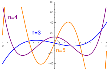
Example 2: We plot some Hermite polynomials and functions.

Plot[{HermiteH[3, x], HermiteH[4, x], Callout[HermiteH[5, x], Style["n=5", 18, Orange], {.2, .35}]}, {x, -2, 2}, PlotRange -> {-50, 70}, PlotStyle -> {{Blue, Thick}, {Purple, Thick}, {Orange, Thick}}, Epilog -> {{Text[Style["n=3", 18, Blue], {-0.7, 20}]}, {Text[ Style["n=4", 18, Purple], {-1.6, 50}]}}]
psi[n_, x_] = Exp[-x^2 /2]*HermiteH[n, x]/Sqrt[2^n *Factorial[n]*Sqrt[Pi]];
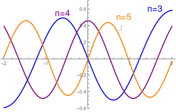
Plot[{psi[3, x], psi[4, x], Callout[psi[5, x], Style["n=5", 18, Orange], {0.8, .35}]}, {x, -2, 2}, PlotRange -> {-0.6, 0.6}, PlotStyle -> {{Blue, Thick}, {Purple, Thick}, {Orange, Thick}}, Epilog -> {{Text[Style["n=3", 18, Blue], {1.6, 0.6}]}, {Text[ Style["n=4", 18, Purple], {-0.6, 0.55}]}}]
     
Hermite polynomials for n = 3, 4, 5.       Hermite functions for n = 3, 4, 5.

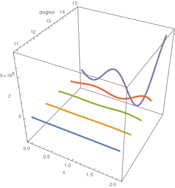
      We can also plot Hermite's polynomials side by side:
f[n_, x_] := HermiteH[n, x];
Table[Plot[f[n, x], {x, 0, 1}], {n, 5, 15}] ParametricPlot3D[ Evaluate@Table[{x, n, f[n, x]}, {n, 11, 15}], {x, 0, 2}, AxesLabel -> {"x", "degree", "z"}, BoxRatios -> 1, PlotRange -> Full, PlotStyle -> Thickness[0.01]]
End of Example 2

As it is seen from the previous example, the Hermite polynomials and functions change from oscillatory behavior to monotonic, exponentially decay at the “turning points." In the vicinity of the turning points, the Hermite functions are approximated in terms of the Airy function, Ai(z),


Fourier transforms


Fourier transform of the Hermite functions are given in the following

Lemma 1: The Hermite functions are eigenfunctions for the Fourier transform in 𝔏²(ℝ):
\[ ℱ_{x\to\xi} \left[ \psi_n (x) \right] (\xi ) = \mbox{P.V.} \int_{-\infty}^{\infty} e^{{\bf j}x\xi} \psi_n (x)\,{\text d}x = {\bf j}^n \sqrt{2\pi}\,\psi_n (\xi ) . \]

We check with Mathematica for n = 6,7,8.

Integrate[ Exp[-x^2/2]*HermiteH[6, x]*Exp[I*x*t], {x, -Infinity, Infinity}]
8 E^(-(t^2/2)) Sqrt[2 \[Pi]] (15 - 90 t^2 + 60 t^4 - 8 t^6)
FourierTransform[Exp[-x^2/2]*HermiteH[7, x], x, t]
-16 I E^(-(t^2/2)) t (-105 + 210 t^2 - 84 t^4 + 8 t^6)
Assuming[t > 0, Integrate[ Exp[I*x*t]*HermiteH[8, x]*Exp[-x^2/2], {x, -Infinity, Infinity}]]
6 E^(-(t^2/2)) Sqrt[ 2 \[Pi]] (105 - 840 t^2 + 840 t^4 - 224 t^6 + 16 t^8)
However
\[ \mbox{P.V.} \int_{-\infty}^{\infty} e^{{\bf j}x\xi} H_n (x)\, e^{-x^2} {\text d} x = {\bf j}^n \sqrt{\pi} \,\xi^n e^{-\xi^2 /4} , \qquad n\in \mathbb{N} = \{ 0,1,2,\ldots \} , \]
Assuming[t > 0, Integrate[ Exp[I*x*t]*HermiteH[8, x]*Exp[-x^2], {x, -Infinity, Infinity}]]
E^(-(t^2/4)) Sqrt[\[Pi]] t^8
and
\[ \mbox{P.V.} \int_{-\infty}^{\infty} e^{{\bf j}x\xi} He_n (x)\, e^{-x^2 /2} {\text d} x = {\bf j}^n \sqrt{2\pi} \,\xi^n e^{-\xi^2 /2} , \qquad n\in \mathbb{N} = \{ 0,1,2,\ldots \} , \]
Assuming[t > 0, Integrate[ Exp[I*x*t]*HermiteH[7, x/Sqrt[2]]*Exp[-x^2/2], {x, -Infinity, Infinity}]]/2^(7/2)
-I E^(-(t^2/2)) Sqrt[2 \[Pi]] t^7

Lemma 2: The Chebyshev--Hermite functions are eigenfunctions for the scaled Fourier transform in 𝔏²(ℝ):
\[ ℱ_{x\to\xi /2} \left[ h_n (x) \right] \left(\frac{\xi}{2} \right) = \mbox{P.V.} \int_{-\infty}^{\infty} e^{{\bf j}x\xi /2} h_n (x)\,{\text d}x = {\bf j}^n 2\,\sqrt{\pi}\,h_n (\xi ) . \]

We check with Mathematica for n = 5, 6.

h[n_, x_] = Exp[-x^2/4]* HermiteH[n, x/Sqrt[2]]/2^(n/2)/Sqrt[Factorial[n]*Sqrt[2*Pi]];
Simplify[Integrate[Exp[I*x*t/2]*h[5, x], {x, -Infinity, Infinity}]/ h[5, t]]
2 I Sqrt[\[Pi]]
Simplify[Integrate[Exp[I*x*t/2]*h[6, x], {x, -Infinity, Infinity}]/ h[6, t]]
-2 Sqrt[\[Pi]]

Example 3: Let Y = N(μ, σ) be a general Gaussian distribution with mean μ and standard deviation σ. In order to compute the moments of the random variable Y, we rewrite the integral representation of Chebyshev-Hermite polynomial as follows,

\[ He_n ({\bf j}x) \left( -{\bf j} \right)^n = \frac{1}{\sqrt{2\pi}}\int_{-\infty}^{+\infty} z^n e^{- (z - x)^2 /2} {\text d} z = E \left[ Y^n \right] . \]
End of Example 3


Rodrigues formulae and Error Function


Many applications utilize a special function known as the error function:
\[ \mbox{erf}(x) = \frac{2}{\sqrt{\pi}} \int_0^x e^{-t^2} {\text d}t = \frac{2}{\sqrt{\pi}} \sum_{n\ge 0} \frac{(-1)^n x^{2n+1}}{n! \left( 2n+1 \right)}. \]
There is another closely related function --- the complementary error function (erfc) defined as
\[ \mbox{erfc}(x) = 1 - \mbox{erf}(x) = \frac{2}{\sqrt{\pi}} \int_x^{\infty} e^{-t^2} {\text d}t . \]
The name "error function" and its abbreviation erf were proposed by J. W. L. Glaisher in 1871 on account of its connection with "the theory of Probability.

The French banker, mathematician, and social reformer Odile Rodrigues showed in 1816 that a large class of second-order Sturm-Liouville ordinary differential equations (ODEs) had polynomial solutions that could be put in a compact and useful form now generally called Rodrigues formulae.

Hermite polynomials can be defined also via Rodrigues formula:

\[ H_n (x) = \left( -1 \right)^n e^{x^2} \frac{{\text d}^n}{{\text d} x^n} \left( e^{-x^2} \right) = e^{x^2 /2} \left( x- \frac{\text d}{{\text d} x} \right)^n e^{-x^2 /2} = \left( 2x - \frac{\text d}{{\text d}x} \right)^n 1 , \qquad n=0,1,2,\ldots . \tag{E.1} \]
and
\[ He_n (x) = \left( -1 \right)^n e^{x^2 /2} \frac{{\text d}^n}{{\text d} x^n} \left( e^{-x^2/2} \right) = e^{x^2 /4} \left( \frac{x}{2} - \frac{\text d}{{\text d}x} \right)^n e^{-x^2 /4} = \left( x- \frac{\text d}{{\text d} x} \right)^n \cdot 1, \qquad n\in \mathbb{N} . \tag{E.2} \]
Simplify[D[Exp[-x^2], {x, 5}]*Exp[x^2]]
-8 x (15 - 20 x^2 + 4 x^4)
Simplify[D[Exp[-x^2/2], {x, 6}]*Exp[x^2/2]]

From Lemma 1, we derive
\[ \frac{{\text d}^n}{{\text d}x^n} \left( e^{-x^2 /2} \right) = \frac{{\bf j}^n}{\sqrt{2\pi}} \int_{-\infty}^{+\infty} \xi^n e^{-\xi^2 /2} e^{{\bf j}x\xi} {\text d}\xi , \qquad n\in \mathbb{N} = \{ 0,1,2,\ldots \} . \]
Now inserting the previous result in the Rodrigues formula, we find the integral representation of the Chebyshev-Hermite polynomials,
\[ He_n (x) = e^{x^2 /2} \frac{(-{\bf j})^n}{\sqrt{2\pi}} \int_{-\infty}^{+\infty} \xi^n e^{-\xi^2 /2} e^{{\bf j}x\xi} {\text d}\xi , \qquad {\bf j}^2 = -1 . \]

The Rodrigues formula shows that Hermite polynomials are closely related to the error function

\[ H_n (x) = \frac{\sqrt{\pi}}{2} \left( -1 \right)^n e^{x^2} \frac{{\text d}^{n+1}}{{\text d} x^{n+1}} \,\mbox{erf}(x) , \qquad \mbox{erf}(x) = \frac{2}{\sqrt{\pi}} \int_0^x e^{-t^2} {\text d}t . \tag{E.3} \]
Simplify[-Sqrt[Pi]*Exp[x^2 ] * D[Erf[x]/2, {x, 6}]]
8 x (15 - 20 x^2 + 4 x^4)

Also,
\[ He_n (x) = \sqrt{\frac{\pi}{2}}\,(-1)^n e^{x^2/2} \frac{{\text d}^{n+1}}{{\text d} x^{n+1}} \,\mbox{erf}\left( \frac{x}{\sqrt{2}} \right) , \qquad n\in \mathbb{N} . \tag{E.4} \]
Simplify[-Sqrt[Pi/2]*Exp[x^2 /2] * D[Erf[x/Sqrt[2]], {x, 6}]]
x (15 - 10 x^2 + x^4)

For Hermite functions, we have

\begin{align*} \psi_n (x) &= \left( 2^n n! \,\sqrt{\pi} \right)^{-1/2} (-1)^n e^{x^2 /2} \,\frac{{\text d}^n}{{\text d} x^n} \left( e^{-x^2} \right) \\ &= \| H_n \|^{-1} (-1)^n \frac{\sqrt{\pi}}{2} \, e^{x^2 /2} \,\frac{{\text d}^{n+1}}{{\text d} x^{n+1}} \, ,\mbox{erf}(x) , \quad n\in \mathbb{N} . \tag{E.5} \end{align*}

Correspondingly, for Chebyshev--Hermite functions, we get
\begin{align*} h_n (x) &= (-1)^n \left( n! \,\sqrt{2\pi} \right)^{-1/2} e^{x^2 /4} \frac{{\text d}^n}{{\text d} x^n} \left( e^{-x^2 /2} \right) \\ &= \| He_n \|^{-1} \sqrt{\frac{\pi}{2}} \, (-1)^n e^{x^2 /4} \,\frac{{\text d}^{n+1}}{{\text d} x^{n+1}} \, \mbox{erf}\left( \frac{x}{\sqrt{2}} \right) , \qquad n\in \mathbb{N} . \tag{E.6} \end{align*}

Here
\[ \| H_n \| = \left( 2^n n! \,\sqrt{\pi} \right)^{1/2} , \qquad \| He_n \| = \left( n! \,\sqrt{\pi} \right)^{1/2} , \qquad n\in \mathbb{N} . \]
Lemma 3: The erroe function is an odd function and
\[ \mbox{erf}(x) = \frac{\sqrt{\pi}}{2} \sum_{n=0}^{\infty} \frac{(-1)^n}{n! \left( 2n+1 \right)} \, x^{2n+1} = \frac{\sqrt{\pi}}{2} \,e^{-x^2}\sum_{n\ge 0} \frac{2^n}{(2n+1)!!}\,x^{2n+1} , \]
where (2n+1)!! = (2n+1)(2n−1)···1 is double factorial.
Using Maclaurin series, we get
\begin{align*} \mbox{erf}(x) &= \frac{2}{\sqrt{\pi}} \int_0^{\infty} - \frac{2}{\sqrt{\pi}} \int_x^{+\infty} e^{-t^2} {\text d} t \\ &= 1 - \frac{2}{\sqrt{\pi}} \int_0^{+\infty} e^{-\left( s + x \right)^2} {\text d} s \\ &= 1 - \frac{2}{\sqrt{\pi}} e^{-x^2} \int_0^{+\infty} e^{-2xs - s^2^2} {\text d} s \\ &= 1 - \frac{2}{\sqrt{\pi}} e^{-x^2} \sum_{n\ge 0} \frac{(-1)^n 2^n}{n!}\, x^n \int_0^{\infty} s^n e^{-s^2} {\text d} s \\ &= 1 - \frac{2}{\sqrt{\pi}} e^{-x^2} \sum_{n\ge 0} \frac{(-1)^n 2^n}{n!}\, x^n \Gamma \left( \frac{n+1}{2} \right) , \end{align*}
where Γ(z) is Euler's gamma function. On the other hand, the parity of the error function gives
\[ \mbox{erf}(x) = - \mbox{erf}(-x) = - \left\{ 1 - \frac{2}{\sqrt{\pi}} e^{-x^2} \sum_{n\ge 0} \frac{2^n}{n!}\, x^{n} \Gamma \left( \frac{n+1}{2} \right) . \]
Then we have
\begin{align*} 2\mbox{erf}(x) &= \frac{1}{\sqrt{\pi}} e^{-x^2} \sum_{n\ge 0} \frac{2^n x^n}{n!} \left[ 1 - (-1)^n \right] \Gamma \left( \frac{n+1}{2} \right) \\ &= \frac{2}{\sqrt{\pi}} e^{-x^2} \sum_{k\ge 0} \frac{2^{2k+1} x^{2k+1}}{(2k+1)!}\, \Gamma (k+1 ) . \end{align*}
Hence, we obtain
\[ \mbox{erf}(x) = \frac{2}{\sqrt{\pi}} e^{-x^2} \sum_{n\ge 0} \frac{2^{2k} k! \,x^{2k+1}}{(2k+1)!} = \frac{2}{\sqrt{\pi}} e^{-x^2} \sum_{k\ge 0} \frac{2^{k} \,x^{2k+1}}{(2k+1)!!} \]

Since

\[ \frac{\text d}{{\text d}x} \,\mbox{erf}(x) = \frac{2}{\sqrt{\pi}} e^{-x^2} , \]
the Hermite function can be rewritten as
\[ \psi_n (x) = \| H_n \|^{-1} \frac{2}{\sqrt{\pi}} \left( -1 \right)^n e^{-x^2} \left( \frac{\text d}{{\text d}x} \right)^{n+1} \mbox{erf}(x) . \]
So we have
\[ \frac{2}{\sqrt{\pi}} \left( \frac{\text d}{{\text d}x} \right)^{n+1} \mbox{erf}(x) = \| H_n \|^{-1} \left( -1 \right)^n e^{-x^2} \psi_n (x) . \]
If n is an odd number, then ψn(0) = 0, and we have
\begin{align*} \left( \frac{\text d}{{\text d}x} \right) \mbox{erf}(x) &= \frac{2}{\sqrt{\pi}} \sum_{n\ge 0} \frac{\| H_n \| \,(-1)^n}{n!}\, \psi_n (0)\,x^n \\ &= \frac{2}{\sqrt{\pi}} \pi^{1/4} \sum_{m\ge 0} \frac{2^m}{\left[ (2m)! \right]^{1/2}}\,\psi_n (0)\, x^{2m} . \end{align*}
Therefore, we have
\[ \mbox{erf}(x) = \frac{2}{\sqrt{\pi}} \pi^{1/4} \sum_{m\ge 0} \frac{2^m}{(2m+1)\left[ (2m)! \right]^{1/2}} \,\psi_{2m} (0)\, x^{2m+1} . \]


Recurrences


Recurrence relations for Hermite polynomials:
\[ H_{n+1} (x) = 2x \,H_n (x) - 2n\,H_{n-1} (x), \qquad n=1,2,\ldots ; \qquad H_0 (x) =1, \quad H_1 (x) =2x . \tag{R.1} \]
Simplify[HermiteH[8, x] - 2*x*HermiteH[7, x] + 14*HermiteH[6, x]]
\[ He_{n+1} (x) = x \,He_n (x) - n\,He_{n-1} (x), \qquad n=1,2,\ldots ; \qquad He_0 (x) =1, \quad He_1 (x) = x . \tag{R.2} \]

Hermite functions can be efficiently computed using a three-term recursion relation from two starting values:

\[ \psi_{n+1} (x) = \sqrt{\frac{2}{n+1}} \,x\,\psi_n (x) - \sqrt{\frac{n}{n+1}}\,\psi_{n-1} (x) , \qquad \psi_0 (x) = \pi^{-1/4} e^{-x^2 /2} , \quad \psi_1 (x) = \pi^{-1/4} \sqrt{2}\,x \,e^{-x^2 /2} . \tag{R.3} \]
psi[n_, x_] = Exp[-x^2 /2]*HermiteH[n, x]/Sqrt[2^n *Factorial[n]*Sqrt[Pi]];
Simplify[psi[9, x] - Sqrt[2/9]*x*psi[8, x] + Sqrt[8/9]*psi[7, x]]
\[ x\,\psi_{n} (x) = \sqrt{(n+1)/2} \,\psi_{n+1} (x) + \sqrt{n/2}\,\psi_{n-1} (x) , \qquad \psi_0 (x) = \pi^{-1/4} e^{-x^2 /2} , \quad \psi_1 (x) = \pi^{-1/4} \sqrt{2}\,x \,e^{-x^2 /2} . \]
Simplify[psi[9, x] - Sqrt[2/9]*x*psi[8, x] + Sqrt[8/9]*psi[7, x]]

Similarly,

\[ x\,h_n (x) = \sqrt{n+1}\,h_{n+1} (x) + \sqrt{n}\, h_{n-1} (x) , \qquad n=1,2,\ldots . \tag{R.4} \]
h[n_, x_] = Exp[-x^2 /4] * HermiteH[n, x/Sqrt[2]]/2^(n/2)/Sqrt[Factorial[n]*Sqrt[2*Pi]];
Simplify[x*h[8, x] - 3*h[9, x] - Sqrt[8]*h[7, x]]
0

Derivatives are expressed via Appell's formula:

\[ \frac{{\text d} H_{n} (x)}{{\text d}x} = 2n\,H_{n-1} (x), \qquad \frac{{\text d} He_{n} (x)}{{\text d}x} = n\,He_{n-1} (x), \qquad n=1,2,\ldots . \tag{R.5} \]
Simplify[D[HermiteH[11, x], x] - 22*HermiteH[10, x]]
In general,
\[ \frac{{\text d}^m H_{n} (x)}{{\text d}x^m} = \frac{2^m n!}{(n-m)!}\, H_{n-m} (x) . \]

Another kind of formulas:
\[ \frac{{\text d} H_{n} (x)}{{\text d}x} = 2x\, H_n (x) - H_{n+1} (x) . \tag{R.6} \]
Simplify[D[HermiteH[11, x], x] - 2*x*HermiteH[11, x] + HermiteH[12, x]]
and
\[ \frac{{\text d} He_{n} (x)}{{\text d}x} = x\,He_n (x) - He_{n+1} (x) = n\,He_{n-1} (x) . \tag{R.7} \]

Example 4: We claim that the convolution of a standard Gaussian distribution with the nth Chebyshev-Hermite polynomial is

\[ \left( \phi \star He_n \right) (x) = \int_{-\infty}^{+\infty} (2\pi )^{-1/2} e^{-(x-t)^2 /2} He_n (t)\,{\text d}t = x^n , \qquad n\in \mathbb{N} = \{ 0,1,2,\ldots \} . \tag{2.1} \]
This means that the convolution yields the moments E[Hen(Y)] of a random variable Y = N(x, 1) with normal distribution. In order to employ the induction, we check Eq.(2.1) for first two values n = 0, 1. Calculations show that
\[ \left( \phi \star He_0 \right) (x) = E \left[ Y^0 \right] = 1, \qquad \left( \phi \star He_1 \right) (x) = E \left[ Y^1 \right] = x. \]
Now we suppose that the statement is true for n − 1,
\[ \left( \phi \star He_{n-1} \right) (x) = \frac{1}{\sqrt{2\pi}} \int_{-\infty}^{+\infty} e^{-(x-t)^2 /2} He_{n-1} (t)\,{\text d} t = x^{n-1} . \tag{2.2} \]
We need to prove it for n to show that
\[ \left( \phi \star He_{n} \right) (x) = \frac{1}{\sqrt{2\pi}} \int_{-\infty}^{+\infty} e^{-(x-t)^2 /2} He_{n} (t)\,{\text d} t = \frac{1}{\sqrt{2\pi}} \int_{-\infty}^{+\infty} e^{-(x-t)^2 /2} \left[ t\,He_{n-1} (t) - He'_{n-1} (t) \right] {\text d} t \]
By integration by parts, we get
\[ \frac{1}{\sqrt{2\pi}} \int_{-\infty}^{+\infty} e^{-(x-t)^2 /2} He'_{n-1} (t)\, {\text d} t = \frac{1}{\sqrt{2\pi}} \int_{-\infty}^{+\infty} e^{-(x-t)^2 /2} \left( x-t \right) He_{n-1} (t)\, {\text d} t \]
Now we took into account that \( \displaystyle e^{-(x-t)^2 /2} \) multiplied by any polynomial of odd degree vanishes. Then
\[ \left( \phi \star He_Ln} \right) (x) = \frac{1}{\sqrt{2\pi}} \int_{-\infty}^{+\infty} e^{-(x-t)^2 /2} He_{n} (t)\,{\text d} t = \frac{x}{\sqrt{2\pi}} \int_{-\infty}^{+\infty} e^{-(x-t)^2 /2} \,He_{n-1} (t) \,{\text d} t . \]
Finally using the induction hypothesis (2.2) in the last expression we obtain the required result.
End of Example 4

For Hermite functions, we have

\[ \frac{{\text d} \psi_{n} (x)}{{\text d}x} = -x\,\psi_{n} (x) + \sqrt{2n}\,\psi_{n-1} (x), \tag{R.8} \]
\[ \frac{{\text d} \psi_{n} (x)}{{\text d}x} = -\sqrt{(n+1)/2}\,\psi_{n+1} (x) + \sqrt{n/2}\,\psi_{n-1} (x), \qquad n=1,2,\ldots . \tag{R.9} \]
Simplify[D[psi[9, x], x] + x*psi[9, x] - Sqrt[18]*psi[8, x]]
From these recurrences, it follows
\[ \left( \frac{\text d}{{\text d}x} + x \right) \psi_n (x) = \sqrt{2n}\,\psi_{n-1} (x) , \qquad \left( x -\frac{\text d}{{\text d}x} \right) \psi_n (x) = \sqrt{2\left( n+1 \right)}\,\psi_{n+1} (x) . \tag{R.10} \]
In particular,
\[ \frac{{\text d} \psi_{0} (x)}{{\text d}x} = - \frac{1}{\sqrt{2}}\, \psi_1 (x) = -x\,\psi_0 (x), \qquad \frac{{\text d} \psi_{1} (x)}{{\text d}x} = \sqrt{2} \left( 1- x^2 \right) \psi_0 (x) . \]

Similarly,
\[ 2\, \frac{{\text d} h_{n} (x)}{{\text d}x} = - \sqrt{n+1}\, h_{n+1} (x) + \sqrt{n}\, h_{n-1} (x) . \tag{R.11} \]
h[n_, x_] = Exp[-x^2 /4] * HermiteH[n, x/Sqrt[2]]/2^(n/2)/Sqrt[Factorial[n]*Sqrt[2*Pi]];
Simplify[2*D[h[8, x], x] + 3*h[9, x] - Sqrt[8]*h[7, x]]
0
and
\[ \left( \frac{\text d}{{\text d}x} + \frac{x}{2} \right) h_n (x) = \sqrt{n}\,h_{n-1} (x) , \qquad \left( \frac{x}{2} -\frac{\text d}{{\text d}x} \right) h_n (x) = \sqrt{n+1}\,h_{n+1} (x) . \tag{R.12} \]

This allows us to find integrals:
\[ \int_{-\infty}^x {\text d} t\,\psi_{n+1} (t) = \sqrt{\frac{2}{n+1}}\,\psi_n (x) + \sqrt{\frac{n}{n+1}} \int_{-\infty}^x {\text d} t\,\psi_{n-1} (t) . \]

For Hermite polynomials, we have
\[ \int_{0}^x {\text d} t\,H_{n} (t) = \frac{1}{2(n+1)} \left[ H_{n+1} (x) - H_{n+1} (0) \right] . \]

Also
\[ \frac{\text d}{{\text d} x} \left[ e^{-x^2} H_n (x) \right] = - e^{-x^2} H_{n+1} (x) , \qquad \frac{\text d}{{\text d} x} \left[ e^{-x^2/2} He_n (x) \right] = - e^{-x^2/e} He_{n+1} (x) . \tag{R.13} \]
ch[n_, x_] = HermiteH[n, x/Sqrt[2]]/2^(n/2);
Simplify[D[Exp[-x^2/2]*ch[5, x], x]*Exp[x^2/2]/ch[6, x]]
-1
Simplify[D[Exp[-x^2]*HermiteH[6, x], x]*Exp[x^2]/HermiteH[7, x]]
-1


Ladder operators


In quantum mechanics, a ladder operator is an operator that increases or decreases the eigenvalue of another operator. Correspondingly, there are two of the ladder operators, known as a raising or creation operator and lowering or annihilation operator. Since we have two orthonomal bases (Hermite functions and Chebyshev--Hermite functions) in Hilbert space 𝔏²(ℝ), we need two kinds of ladder operators. For Hermite functions, we denote them with letter using bold fonts as it is common in mathematics. On the other hand, we utilize letters with hat as they are usually written in physics.

So we define the creation operator as

\[ {\bf a}^{\dagger} = -\texttt{D} + x\texttt{I} = -\frac{\text d}{{\text d}x} + x \]
and its adjoint operator, called the annihilation operator:
\[ {\bf a} = \texttt{D} + x\texttt{I} = \frac{\text d}{{\text d}x} + x , \]
where \( \displaystyle \texttt{D} = {\text d}/{\text d}x , \quad\mbox{and} \quad \texttt{I} = \texttt{D}^0 \quad \) is the identity operator. Then we have
\[ {\bf a}^{\dagger} e^{-x^2 /2} H_n (x) = \left( -\texttt{D} + x \right) e^{-x^2 /2} H_n (x) = \left( 2x\,H_n - H'_n (x) \right) e^{-x^2 /2} . \]
Using the Appell's formula \( H'_n (x) = 2n\,H_{n-1} (x) , \) we get
\[ {\bf a}^{\dagger} e^{-x^2 /2} H_n (x) = \left( x\, H_n (x) - n\,H_{n-1} (x) \right) e^{-x^2 /2} = H_{n+1} (x)\, e^{-x^2 /2} . \]
This leads to
\[ {\bf a}^{\dagger} \psi_n (x) = \sqrt{2 \left( n+1 \right)}\, \psi_{n+1} (x) , \qquad {\bf a}\,\psi_n (x) = \sqrt{2n}\, \psi_{n-1} , \qquad n=0,1,2,\ldots . \tag{L.1} \]
Their compositions are
\[ {\bf a}\,{\bf a}^{\dagger} \psi_n (x) = 2\left( n+1 \right) \psi_n (x) , \qquad {\bf a}^{\dagger} {\bf a}\,\psi_n (x) = 2n\,\psi_n (x) . \tag{L.2} \]
Hence,
\[ \frac{\text d}{{\text d}x} \left[ e^{-x^2} H_n (x) \right] = - e^{-x^2} H_{n+1} (x) , \]
and
\[ \frac{\text d}{{\text d}x} \left[ e^{-x^2 /2} He_n (x) \right] = -e^{-x^2/2} He_{n+1} (x) , \qquad n\in \mathbb{N} . \]
Simplify[D[Exp[-x^2 /2]*HermiteH[n, x/Sqrt[2]], x]/2^(n/2)* Exp[x^2 /2] /. n -> 4]
-x (15 - 10 x^2 + x^4)

Similarly, we have

\[ {\bf a}\, e^{-x^2 /2} H_n (x) = H'_{n} (x)\, e^{-x^2 /2} = 2n\,H_{n-1} (x)\, e^{-x^2 /2} . \]
So
\[ {\bf a}\, \psi_n (x) = \sqrt{2 \,n}\, \psi_{n-1} (x) , \qquad n=0,1,2,\ldots . \]
The operations of differentiation and multiplication by x can also be expressed in terms of the raising and lowering operators:
\begin{align*} x\,\psi_n (x) &= \frac{1}{2} \left( {\bf a} + {\bf a}^{\dagger} \right) \psi_n (x) = \sqrt{n/2}\,\psi_{n-1}(x) + \sqrt{(n+1)/2}\,\psi_{n+1} (x) , \\ \frac{\text d}{{\text d}x}\,\psi_n (x) &= \frac{1}{2} \left( {\bf a} - {\bf a}^{\dagger} \right) \psi_n (x) = \sqrt{n/2}\,\psi_{n-1}(x) - \sqrt{(n+1)/2}\,\psi_{n+1} (x) . \end{align*}

Upon introducing the Hermite differential operator

\[ {\bf h} = \frac{1}{2} \left( {\bf a}\, {\bf a}^{\dagger} + {\bf a}^{\dagger} {\bf a} \right) = -\texttt{D}^2 + x^2 , \]
we get
\[ {\bf h}\, e^{-x^2 /2} H_n (x) = \left( 2n +1 \right) e^{-x^2 /2} H_n (x) . \]

This yields

\[ {\bf h} \psi_n (x) = \left( - \frac{{\text d}^2}{{\text d} x^2} + x^2 \right) \psi_n (x)= \left( 2n+1 \right) \psi_n (x) , \qquad n= 1,2,\ldots . \tag{L.3} \]
psi[n_, x_] = Exp[-x^2 /2]*HermiteH[n, x]/Sqrt[2^n *Factorial[n]*Sqrt[Pi]]; Simplify[-D[psi[8, x], x, x] + (x^2)*psi[8, x] - (2*8 + 1)*psi[8, x]]
0


Example 5:

We introduce a lowering (or annihilation) operator \( \hat{a} \) and a raising, or creation, operator \( \hat{a}^{\ast} \) according to the formulas:

\[ \hat{a} = \frac{1}{\sqrt{2}} \left( x + \frac{{\text d}}{{\text d}x} \right) \qquad \mbox{and} \qquad \hat{a}^{\ast} = \frac{1}{\sqrt{2}} \left( x - \frac{{\text d}}{{\text d}x} \right) . \]
that are adjoint to each other. They obey the commutation relations
\[ \left[ \hat{a} , \hat{a}^{\ast} \right] = \left[ \frac{{\text d}}{{\text d}x} , x \right] =1, \qquad \mbox{and} \qquad \left[ \hat{a} , \hat{a} \right] = 0 = \left[ \hat{a}^{\ast} , \hat{a}^{\ast} \right] . \]
Let us introduce the Hermitian number operator \( N= \hat{a}^{\ast} \hat{a} \) and the Hamiltonian
\[ {\cal H} = N + \frac{1}{2} = \hat{a}^{\ast} \hat{a} + \frac{1}{2} = \frac{1}{2} \left( \hat{a}^{\ast} \hat{a} + \hat{a} \hat{a}^{\ast} \right) . \]
Let \( |n\rangle \) be an eigenfunction of \( {\cal H} : \ {\cal H} \,|n\rangle = \lambda_n |n\rangle , \) whose eigenvalue λn is unknown at this point. Now we prove the key property that N has nonnegative integer eigenvalues:
\[ N \, |n\rangle = \left( \lambda_n - \frac{1}{2} \right) |n\rangle = n\, |n\rangle , \qquad n=0,1,2,\ldots , \]
that is, \( \lambda_n = n + 1/2 . \) Since \( \hat{a} |n\rangle \) is complex conjugate to \( \langle n | \hat{a}^{\ast} , \) the normalization integral \( \langle n | \hat{a}^{\ast} \, \hat{a} |n\rangle \ge 0 \) and is finite. From
\[ \left( \hat{a} |n\rangle \right)^{\ast} \hat{a} |n\rangle = \langle n | \hat{a}^{\ast} \, \hat{a} |n\rangle = \left( \lambda_n - \frac{1}{2} \right) \ge 0 , \]
we see that N has nonnegative eigenvalues.

Using commutation relations

\[ \left[ N, \hat{a}^{\ast} \right] = \hat{a}^{\ast} , \qquad \left[ N, \hat{a} \right] = -\hat{a} , \]
and \( \hat{a} \, \hat{a}^{\ast} = N + \left[ \hat{a}, \hat{a}^{\ast} \right] = N+1 , \) we find that
\begin{align*} N \left( \hat{a}^{\ast}\, |n\rangle \right) &= \hat{a}^{\ast} \left( \hat{a} \, \hat{a}^{\ast} \right) |n\rangle = \hat{a}^{\ast} \left( \left[ \hat{a}, \hat{a}^{\ast} \right] + N \right) |n\rangle \\ &= \hat{a}^{\ast} \left( N+1 \right) |n\rangle = \left( \lambda_n + \frac{1}{2} \right)= (n+1) \hat{a}^{\ast}\, |n\rangle = (n+1) \,\hat{a}^{\ast}\, |n\rangle , \\ N \left( \hat{a}\, |n\rangle \right) &= \left( \hat{a}, \hat{a}^{\ast} -1 \right) |n\rangle = \hat{a} \left( N-1 \right) |n\rangle = \left( n-1 \right) |n\rangle . \end{align*}
In other words, N acting on \( \hat{a} \,|n\rangle \) shows that \( \hat{a} \) has lowered the eigenvalue n by one unit; hence it is a lowering (or annihilation) operator. Similarly, N acting on \( \hat{a}^{\ast} \,|n\rangle \) shows that \( \hat{a}^{\ast} \) has raised the eigenvalue n corresponding to \( |n \rangle \)  by one unit, whence its name raising, or creation, operator. Therefore,
\[ \hat{a} |n\rangle \, \sim |n-1 \rangle , \qquad \hat{a}^{\ast} |n\rangle \,\sim\, |n+1 \rangle . \]
Applying \( \hat{a} \) repeatedly, we can reach all lower states, including the lowest, or ground, state \( |0\rangle , \) with eigenvalue λ0. We cannot step lower because \( \lambda_0 \ge 0. \) Hence, \( \hat{a}\,|0\rangle \equiv 0, \) suggesting we construct \( \psi_0 = | 0 \rangle \) from the (factored) first-order ODE
\[ \sqrt{2}\,\hat{a} \, \psi_0 = \left( \frac{\text d}{{\text d}x} +x \right) \psi_0 =0 . \]
Integrating
\[ \frac{\psi_0'}{\psi_0} = -x, \]
we obtain
\[ \ln \, \psi_0 (x) = -\frac{x^2}{2} , \]
where c0 is an integration constant. The solution
\[ \psi_0 (x) = c_0 e^{-x^2 /2} . \]
is a Gaussian that can be normalized, with \( c_0 = \pi^{-1/4} , \) using the error integral. Using ψ0, we find
\[ {\cal H} \,|0\rangle = \left( \hat{a}^{\ast}\hat{a} + \frac{1}{2} \right) |0\rangle = \frac{1}{2}\,|0\rangle . \]
So its energy eigenvalue is \( \lambda_0 = 1/2 , \) and its number eigenvalue is n = 0, confirming the notation \( |0\rangle . \) Applying \( \hat{a}^{\ast} \) repeatedly to \( \psi_0 = |0\rangle , \) all other eigenvalues are confirmed to be \( \lambda_n = n+1/2 . \) Using normalizations, we find
\[ \left\langle \,\vert \hat{a} \,\hat{a}^{\ast} \vert n \right\rangle = \left\langle \,\vert \hat{a}^{\ast} \,\hat{a} +1 \vert n \right\rangle = n+1 , \]
showing
\[ \sqrt{n+1}\,|n+1 \rangle = \hat{a}^{\ast} \vert n \rangle , \qquad \sqrt{n}\,|n-1\rangle = \hat{a} \vert n \rangle . \]
Thus, the excited-state wave functions, ψ1, ψ2, and so on, are generated by the raising operator
\[ |1 \rangle = \hat{a}^{\ast} \vert 0 \rangle = \frac{1}{\sqrt{2}} \left( x-\frac{\text d}{{\text d}x} \right) \psi_0 = \frac{x\sqrt{2}}{\pi^{1/4}} \, e^{-x^2 /2} , \]
yielding
\[ \psi_n (x) = N_n H_n (x) \,e^{-x^2 /2} , \qquad N_n = \pi^{-1/4} \left( 2^n n! \right)^{-1/2} . \]
End of Example 5

We introduce a lowering (or annihilation) operator \( \hat{a} \) and a raising, or creation, operator \( \hat{a}^{\ast} \) according to the formulas:

\[ \hat{a} = \frac{x}{2} + \frac{{\text d}}{{\text d}x} \qquad \mbox{and} \qquad \hat{a}^{\ast} = \frac{x}{2} - \frac{{\text d}}{{\text d}x} , \]
that are adjoint to each other. They obey the commutation relations
\[ \left[ \hat{a} , \hat{a}^{\ast} \right] = \left[ \frac{{\text d}}{{\text d}x} , x \right] =1, \qquad \mbox{and} \qquad \left[ \hat{a} , \hat{a} \right] = 0 = \left[ \hat{a}^{\ast} , \hat{a}^{\ast} \right] . \]
From Eq.(R.12), it follows
\[ \hat{a}\, h_n (x) = \sqrt{n}\,h_{n-1} , \qquad \hat{a}^{\ast} h_n (x) = \sqrt{n+1}\,h_{n+1} , \qquad n \in \mathbb{N} . \tag{L.4} \]
Upon introducing the Hamiltonian operator \( \displaystyle \hat{H} = \frac{1}{2} \left( \hat{a}\,\hat{a}^{\ast} + ,\hat{a}^{\ast} \hat{a} \right) , \) we derive
\[ \hat{H} \, h_n (x) = \left( \frac{x^2}{4} - \frac{{\text d}^2}{{\text d}x^2} \right) h_n (x) = \frac{2n+1}{2}\,h_n (x) , \qquad n\in \mathbb{N} . \tag{L.5} \]
h[n_, x_] = Exp[-x^2 /4] * HermiteH[n, x/Sqrt[2]]/2^(n/2)/Sqrt[Factorial[n]*Sqrt[2*Pi]];
Simplify[-D[h[8, x], x, x] + (x^2/4)*h[8, x] - (2*8 + 1)/2*h[8, x]]
0

Example 6: The harmonic oscillator is almost ubiquitous model system in any field of physics. Here we present a fairly solid and pedagogically effective way to treat the quantum harmonic oscillator. It is one of the few problems that can really be solved in closed form, and is a very generally useful solution, both in approximations and in exact solutions of various problems.

As t was discussed in tutirial I (see section viii), a harmonic oscillator is a model that describes a particle of mass m moving in a single direction and subject to a restoring force that is proportional to the displacement of the particle (also is known as Hooke's law). In classical Newtonian mechanics this means that the acting force is proportional to the displacement x:

\[ F = m\,a = m\,\frac{{\text d}v}{{\text d}t} = -k\,x , \]
where \( \displaystyle v = \dot{x} = {\text d}x/{\text d} t \) is the velocity of the particle and k is a positive number, characteristic of the resistance; it is called the force constant or spring constant. This constant coefficient differential equation has the general solution:
\[ x(t) = c_1 \cos \left( \omega t \right) + c_2 \sin \left( \omega t \right) , \qquad \omega = +\sqrt{\frac{k}{m}} , \]
where c₁ and c₂ are arbitrary real numbers. Here ω is the angular frequency. Multiplying both sides of the governing equation by v, we obtain
\[ m\,\frac{{\text d}v}{{\text d}t} \,v + k\,x\,v = 0 \qquad \iff \qquad \frac{{\text d}}{{\text d}t} \left[ \frac{m}{2}\,v^2 + \frac{k}{2}\, x^2 \right] = 0 . \]
The expression inside brackets is known as the Hamiltonian for this simple one-dimensional system:
\[ H(v, x) = \frac{m}{2}\,v^2 + \frac{k}{2}\, x^2 . \]
It is actually the total energy E of an oscillator that is the sum of its kinetic energy K = mv²/2 and the elastic potential energy of the force. Since mass m of the particle does not depend on time t, it is convenient to introduce the momentum: p = mv instead of velocity. Then the coresponding Hamiltonian is interpreted as the sum a kinetic energy term, K, and a potential energy term, Π:
\[ H(p,q) = K + \Pi = \frac{1}{2m}\, p^2 + \frac{k}{2}\, q^2 , \]
where q corresponds to displacement (in some coordinate system) and p = mv. Remembering from tutorial I that k/m = ω², where ω is characteristic angular frequency of this system, we can rewite the Hamiltonian as
\[ H(p,q) = \frac{1}{2m}\, p^2 + \frac{m\,\omega^2}{2}\, q^2 , \qquad \omega = + \sqrt{\frac{k}{m}} . \tag{6.1} \]


In quantum mechanics, the harmonic motion begins with the specification of the Schrödinger equation
\[ {\bf j} \hbar \,\partial_t \Psi = \hat{H} \left( \hat{p}, \hat{q} \right) \Psi , \qquad \mbox{with} \quad {\bf j}^2 = -1, \]
where ℏ ≈ 1.054571817... × 10−34 [joule·second = m² kg /s] is the reduced Planck constant, and the Hamiltoniam operator is the sum of a kinetic energy term, K, and a potential energy term, Π (Greek letter "p" in upper case):
\[ \hat{H}\left( \hat{p} , \hat{q} \right) = K + \Pi = \frac{1}{2m}\,\hat{p} + \frac{k}{2}\,\hat{q} , \]
where \( \displaystyle \quad \hat{p} = -{\bf j}\hbar\,\partial_x \quad \) is the momentum operator in the x-direction, and \( \displaystyle \quad \hat{q} \) is the position operator. Here Ψ is the wavefunction that is associated energies for this system, and m is an effective (reduced) mass, and k is an effective force constant. For a diatomic molecule, there is only one vibrational mode, so there will be only a single set of vibrational wavefunctions with associated energies for this system.

Substituting the definitions for the operators yields

\[ \hat{H}(q) = -\frac{\hbar^2}{2m}\,\frac{{\text d}^2}{{\text d}q^2} + \frac{k}{2}\,q^2 . \]

This Hamiltonian appears in various applications, and in fact the approximation of the harmonic oscillator is valid near the minimum of any potential function. Application of separation of variables to the Schrödinger equation, Ψ = T(t) w(x), we obtain

\[ {\bf j} \hbar \,\partial_t \,T(t)\,w(x) = T(t)\,\hat{H}(x)\,w(x) \qquad \Longrightarrow \qquad \frac{{\bf j} \hbar \,\partial_t \,T(t)}{T(t)} = \frac{\hat{H}\,w(x)}{w(x)} = E , \]
where E is a separation constant. This leads to the time-independent Schrödinger equation
\[ - \frac{\hbar^2}{2m}\,\frac{{\text d}^2 w}{{\text d}x^2} + \frac{k}{2}\,x^2 w = E\,w , \]
or upon rearranging
\[ \frac{{\text d}^2 w}{{\text d}x^2} + \frac{2m}{\hbar^2}\left( E - \frac{k}{2}\,x^2 \right) w = 0 . \tag{6.1} \]
This differential equation is not straightforward to solve. Rather than fully develop the details of the solution, we will introduce dimensionless variables because it is not good to carry around so many constants in that equation. Therefore, we make substitution
\[ \xi = \frac{x}{\beta} \qquad \mbox{or} \qquad x = \beta\,\xi , \]
where β has length unit that makes ξ dimensionless constant. Using cbange variables rule
\[ \frac{{\text d}^2}{{\text d}x^2} = \frac{1}{\beta^2}\cdot \frac{{\text d}^2}{{\text d}\xi^2} , \]
this substitution yields
\[ \frac{1}{\beta^2} \cdot\frac{{\text d}^2 w}{{\text d}\xi^2} + \frac{2m}{\hbar^2}\, E - \frac{m\,k}{\hbar^2}\,\xi^2 \beta^2 w = 0 . \]
Upon multiplication by β², we get
\[ \frac{{\text d}^2 w}{{\text d}\xi^2} + \frac{2m}{\hbar^2}\,\beta^2 E - \frac{m\,k}{\hbar^2}\,\xi^2 \beta^4 w = 0 . \tag{6.2} \]
Now we choose the value of constant β in Eq.(6.2) so that the multiple of ξ² will be a constant, which we denote by κ². This yields
\[ \frac{{\text d}^2 w}{{\text d}\xi^2} + \frac{2m}{\hbar^2}\,\beta^2 E - \kappa^2\,\xi^2 w = 0 , \qquad \beta^2 = \kappa\,\frac{\hbar}{\sqrt{m\,k}} . \tag{6.3} \]
In order to simplify the expression for β, we revoke angula velocity from classical harmonic oscillator:    ω² = k/m. This gives a standard Sturm--Liouville problem
\[ \frac{{\text d}^2 w}{{\text d}\xi^2} + \lambda\,w - \kappa^2\,\xi^2 w = 0 , \qquad \lambda = \frac{2\kappa}{\hbar\omega}\, E , \quad \beta^2 = \kappa\,\frac{\hbar}{m\omega} . \tag{6.4} \]
1
End of Example 6

Example 7: We consider Sturm--Liouville problem for harmonic oscillator (6.4) from the previous example in case when κ = 1:

\[ \frac{{\text d}^2 w}{{\text d}\xi^2} + \lambda\,w - \xi^2 w = 0 , \qquad \lambda = \frac{2}{m\omega}\, E , \quad \beta^2 = \frac{\hbar}{m\omega} . \tag{7.1} \]
We are looking for nontrivial solutions of Eq.I7.1) that belong to 𝔏²(−∞, ∞). We know that this problem has discrete number of eigenvalues λn = (2n+1),   n = 0, 1, 2, …. The corresponding eigenfunctions are Hermite functions:
\[ \lambda_n = (2n+1) = \frac{2m}{\hbar^2}\,E_n \qquad \Longrightarrow \qquad E_n = \left( 2n+1 \right) \frac{\hbar \omega}{2}, \quad n=0,1,2,\ldots . \tag{7.2} \]
The corresponding eigenfunctions are
\[ w_n (x) = \psi_n \left( x\,\sqrt{\frac{m\omega}{\hbar}} \right) = \left( \frac{m\omega}{\pi\hbar} \right)^{1/4} \frac{1}{\sqrt{2^n n!}} \,H_n \left[ \left( \frac{m\omega}{\hbar} \right)^{1/2} x\right] \exp\left\{ - \frac{m\omega}{2\hbar}\,x^2 \right\} , \qquad n \in \mathbb{N}. \tag{7.3} \]

Example 8: We consider Sturm--Liouville problem for harmonic oscillator (6.4) from the previous example in case when κ = ½:

\[ \frac{{\text d}^2 w}{{\text d}\xi^2} + \lambda\,w - \frac{\xi^2}{4}\, w = 0 , \qquad \lambda = \frac{1}{m\omega}\, E , \quad \beta^2 = \frac{\hbar}{2m\omega} . \tag{8.1} \]
We are looking for nontrivial solutions of Eq.I7.1) that belong to 𝔏²(−∞, ∞). We know that this problem has discrete number of eigenvalues λn = n+½,   n = 0, 1, 2, …. The corresponding eigenfunctions are Chebyshev--Hermite functions:
\[ \lambda_n = n+\frac{1}{2} = \frac{2m}{\hbar^2}\,E_n \qquad \Longrightarrow \qquad E_n = \left( 2n+1 \right) \frac{\hbar \omega}{2}, \quad n=0,1,2,\ldots . \tag{8.2} \]
The corresponding eigenfunctions are
\[ w_n (x) = h_n \left( x\,\sqrt{\frac{2m\omega}{\hbar}} \right) = \left( \frac{m\omega}{\pi\hbar} \right)^{1/4} \frac{1}{\sqrt{n!}} \,He_n \left[ \left( \frac{2m\omega}{\hbar} \right)^{1/2} x\right] \exp\left\{ - \frac{m\omega}{2\hbar}\,x^2 \right\} , \qquad n \in \mathbb{N}. \tag{8.3} \]


Sturm--Liouville problems


The Hermite polynomials or Chebyshev--Hermite polynomials are solutions of the differential equations
\[ \frac{\text d}{{\text d}x} \left( e^{-x^2} \frac{{\text d}y}{{\text d}x}\right) + 2n\, e^{-x^2} y = 0 \qquad \mbox{or} \qquad y'' -2x\,y' + 2n\, y =0 , \qquad y= H_n (x), \tag{SL.1} \]
and
\[ \frac{\text d}{{\text d}x} \left( e^{-x^2 /2} \frac{{\text d}y}{{\text d}x}\right) + n\, e^{-x^2 /2} y = 0 \qquad \mbox{or} \qquad y'' -x\,y' + n\, y =0 , \qquad y= He_n (x), \tag{SL.2} \]
respectively.

Hermite polynomials Hn(x) are eigenfunctions of the Sturm--Liouville problem for the Hermite differential equation on the infinite interval \( (-\infty , \infty ) : \)
\[ y'' -2x\,y' + \lambda\,y =0 , \qquad \mbox{or} \qquad \frac{{\text d}}{{\text d}x} \left( e^{-x^2} \, \frac{{\text d}y}{{\text d}x} \right) + \lambda e^{-x^2}\, y =0, \tag{SL.3} \]
subject to the condition that its solutions grow at infinity no faster than a polynomial, corresponding to eigenvalues \( \lambda_n = 2n \ge 0, \) an integer.

The Chebyshev--Hermite polynomials Hen(x) are eigenfunctions corresponding to eigenvalues λ = n of the Sturm--Liouville problem for the Hermite differential equation on the infinite interval \( (-\infty , \infty ) : \)

\[ y'' -x\,y' + \lambda\,y =0 , \qquad \lambda = n , \qquad \lambda = 2n , \qquad n,1,2,\ldots . \tag{SL.4} \]
The eigenvalue problems for both, the Hermite and Chebyshev--Hermite polynomials, include requirement that solution must grow no faster than a polynomial.

The Hermite functions are the eigenfunctions of the elliptic operator \( - \frac{{\text d}^2}{{\text d} x^2} + x^2 . \) These functions are solutions to the differential equation that involves a quantum mechanical, simple harmonic oscillator:

\[ \psi''_n (x) + \left( 2n +1-x^2 \right) \psi_n (x) =0, \qquad n=0,1,2,\ldots \tag{SL.5} \]
Also,
\[ \left( \frac{x^2}{4} - \frac{{\text d}^2}{{\text d} x^2} \right) h_n (x) = \frac{2n+1}{2}\, h_n (x) , \qquad n \in \mathbb{N} = \{ 0,1,2,\ldots \} . \tag{SL.6} \]


Useful Formulas


Hermite polynomials admits a symmetry relation:

\[ H_n (-x) = (-1)^n \,H_n (x) , \qquad He_n (-x) = (-1)^n He_n (x) , \qquad n=0,1,2,\ldots . \]

The Hermite polynomials evaluated at zero argument are called Hermite numbers.

\[ H_n (0) = \begin{cases} (-1)^{n/2} 2^{n/2} \,(n-1)!! , & \quad \mbox{if $n$ is even}, \\ 0 , & \quad \mbox{if $n$ is odd,} \end{cases} \qquad n=0,1,2,\ldots \]
\[ He_n (0) = \begin{cases} (-1)^{n/2} 2^{-n/2} /(n)! , & \quad \mbox{if $n$ is even}, \\ 0 , & \quad \mbox{if $n$ is odd,} \end{cases} \qquad n=0,1,2,\ldots \]
In particular,
\[ H_{2m} (0) = (-1)^m \frac{(2m)!}{m!} = (-1)^m 2^m \left( 2m-1 \right)!! , \qquad H_{2m+1} (0) = 0 ; \]
and
\[ H'_{2m} (0) = 0, \qquad H'_{2m+1} (0) = (-1)^m 2\,\frac{(2m+1)!}{m!} . \]
The antiderivative is
\[ \int_0^x H_n (t)\,{\text d}t = \frac{H_{n+1} (x) - H_{n+1} (0)}{2\left( n+1 \right)} . \]
Lemma 4: For any nonnegative integer m, we have
\[ \int_{\mathbb{R}} x^m e^{-x^2} {\text d} x = \frac{1 + (-1)^m}{2}\, \Gamma \left( \frac{m+1}{2} \right) , \qquad \int_0^{\infty} x^m e^{-x^2} {\text d} x = \frac{1}{2}\,\Gamma \left( \frac{m+1}{2} \right) \]
Assuming[p > 0, Integrate[Exp[-x^2]*x^p, {x, -Infinity, Infinity}]]
1/2 (1 + (-1)^p) Gamma[(1 + p)/2]
Assuming[p > 0, Integrate[Exp[-x^2]*x^p, {x, 0, Infinity}]]
1/2 Gamma[(1 + p)/2]
Similarly,
Lemma 5: For any nonnegative integer m, we have
\[ \int_{\mathbb{R}} x^m e^{-x^2 /2} {\text d} x = 2^{(m-1)/2}\left[ 1 + (-1)^m \right] \Gamma \left( \frac{m+1}{2} \right) , \qquad \int_0^{\infty} x^m e^{-x^2 /2} {\text d} x = 2^{(m-1)/2}\,\Gamma \left( \frac{m+1}{2} \right) \]
Assuming[p > 0, Integrate[Exp[-x^2/2]*x^p, {x, -Infinity, Infinity}]]
2^(1/2 (-1 + p)) (1 + (-1)^p) Gamma[(1 + p)/2]
Assuming[p > 0, Integrate[Exp[-x^2/2]*x^p, {x, 0, Infinity}]]
2^(1/2 (-1 + p)) Gamma[(1 + p)/2]


  1. Hermite Functions, Springer.
  2. Kagawa, T.: Hermite function expansions of Heaviside function. Journal of Pseudo-Differential Operators and Applications, 2015, 6, No. 1, pp. 21–32.
  3. Kagawa, T. & Yoshino, K., The Hermite expansion of the characteristic functions, Journal of Pseudo-Differential Operators and Applications, 2017, Vol. 8, No. 2, pp. 255–273. https://doi.org/10.1007/s11868-017-0188-x
  4. Sadlok, Z. On Hermite expansion of x^p, Annales Polonici mathematici, 1980, 38, pp. 159--162. doi: 10.4064/ap-38-2-159-162
  5. Thangavelu, S., Lectures on Hermite and Laguerre Expansions Mathematical Notes, 42. Princeton University Press, Princeton, New Jersey, 1993.


Return to Mathematica page

Return to the main page (APMA0340)
Return to the Part 1 Matrix Algebra
Return to the Part 2 Linear Systems of Ordinary Differential Equations
Return to the Part 3 Non-linear Systems of Ordinary Differential Equations
Return to the Part 4 Numerical Methods
Return to the Part 5 Fourier Series
Return to the Part 6 Partial Differential Equations
Return to the Part 7 Special Functions