Preface


An elliptic function is a function meromorphic on the complec plane ℂ that is periodic in two directions. Elliptic integrals were first encountered by John Wallis around 1655. Historically, elliptic functions were first discovered by Niels Henrik Abel (1802--1829) as inverse functions of elliptic integrals. However, their theory was developed by the German mathematician Carl Gustav Jacob Jacobi (1804--1851), who called December 23, 1751 the birthday of elliptic functions, because on that day Euler (1017--1783) was asked his opinion of a paper by Fagnano (1715--1797) on arcs of lemniscates.

There are known two standard forms of elliptic functions: Jacobi elliptic functions and Weierstrass elliptic functions. Jacobi elliptic functions arise as solutions to differential equations of the form

\[ \frac{{\text d}^2 x}{{\text d} t^2} = a + b\,x + c\,x^2 + d\,x^3 , \]
and Weierstrass elliptic functions arise as solutions to differential equations of the form
\[ \frac{{\text d}^2 x}{{\text d} t^2} = a + b\,x + c\,x^2 . \]

Return to computing page for the first course APMA0330
Return to computing page for the second course APMA0340
Return to Mathematica tutorial for the first course APMA0330
Return to Mathematica tutorial for the second course APMA0340
Return to the main page for the first course APMA0330
Return to the main page for the second course APMA0340
Return to Part VII of the course APMA0340
Introduction to Linear Algebra with Mathematica


Incomplete elliptic integrals


There are known four incomplete elliptic integrals: \begin{align} F (\phi , k ) &= \int_0^{\phi} \frac{{\text d}\theta}{\sqrt{1 - k^2 \sin^2 \theta}} = \int_0^{\sin\phi} \frac{{\text d}t}{\sqrt{1 - t^2} \,\sqrt{1 - k^2 t^2}} , \label{elliptic.1} \\ E (\phi , k ) &= \int_0^{\phi} \sqrt{1 - k^2 \sin^2 \theta}\,{\text d}\theta = \int_0^{\sin\phi} \frac{\sqrt{1 - k^2 t^2}}{\sqrt{1- t^2}}\,{\text d}t , \label{elliptic.2} \\ D (\phi , k ) &= \int_0^{\phi} \frac{\sin^2 \theta \,{\text d}\theta}{\sqrt{1 - k^2 \sin^2 \theta}} = \int_0^{\sin\phi} \frac{t^2 {\text d}t}{\sqrt{1 - t^2} \,\sqrt{1 - k^2 t^2}} = \frac{1}{k^2} \left[ F(\phi , k) - E (\phi , k) \right] , \label{elliptic.3} \\ \Pi (\phi , \alpha^2 , k ) &= \int_0^{\phi} \frac{{\text d}\theta}{\sqrt{1 - k^2 \sin^2 \theta} \left( 1 - \alpha^2 \sin^2 \theta \right)} = \int_0^{\sin\phi} \frac{{\text d}t}{\sqrt{1- t^2} \,\sqrt{1 - k^2 t^2} \left( 1 - \alpha^2 t^2 \right)} . \label{elliptic.4} \end{align} The cases with ϕ = π/2 are known as the complete integrals: \begin{align} & \quad {\bf complete }\ {\bf elliptic } \ {\bf integral }\ {\bf of }\ {\bf the }\ {\bf first }\ {\bf kind:} \notag \\ K(k) &= F \left( \frac{\pi}{2} , k \right) = \int_0^1 \frac{{\text d}t}{\sqrt{1- t^2}\,\sqrt{1 - k^2 t^2}} , \label{elliptic.5} \\ & \quad {\bf complete }\ {\bf elliptic } \ {\bf integral }\ {\bf of }\ {\bf the }\ {\bf second }\ {\bf kind:} \notag \\ E(k) &= E\left( \frac{\pi}{2} , k \right) = \int_0^1 \sqrt{\frac{1 - k^2 t^2}{1-t^2}} \,{\text d}t , \label{elliptic.6} \\ D(k) &= D \left( \frac{\pi}{2} , k \right) = \frac{1}{k^2} \left[ K(k) - E(k) \right] , \label{elliptic.7} \\ & \quad {\bf complete }\ {\bf elliptic } \ {\bf integral }\ {\bf of }\ {\bf the }\ {\bf third }\ {\bf kind:} \notag \\ \Pi \left( \alpha^2 k \right) &= \Pi \left( \frac{\pi}{2} , \alpha^2 , k \right) . \label{elliptic.8} \end{align} Mathematica has dedicated commands for evaluating elliptic integrals:
EllipticK[ m ]
EllipticE[ m ]
EllipticPi[ n, m ]

     
Plot[{Callout[ElliptiK[m], "EllipticK(m)", Left, Frame -> True, FrameMargins -> 10], Callout[EllipticE[m], "EllipticE(m)", Right, Frame -> True, CalloutStyle -> Yellow], Callout[(EllipticK[m] - EllipticE[m])/m^2, "EllipticD(m)", Above, Frame -> True, Background -> Pink]}, {m, -1, 1}, PlotStyle -> Thickness[0.01]]
       Complete elliptic functions K(m), E(m), and D(m).            Mathematica code

     
Plot3D[EllipticPi[n, m], {n, -1, 1}, {m, -1, 1}, PlotStyle -> Directive[Orange, Specularity[White, 40]]]
       Elliptic integral of the third kind Π(n, m).            Mathematica code

Using the binomial series

\[ \left( 1 - m\,\sin^2 \theta \right)^{-1/2} = \sum_{n\ge 0} \frac{(2n-1)!!}{(2n)!!}\, m^n \sin^{2n} \theta = 1 + \frac{1}{2}\,m\,\sin^2 \theta + \frac{3}{8}\,m^2 \sin^4 \theta + \cdots , \]
and the integral
\[ \int_0^{\pi /2} \sin^{2n} \theta \,{\text d}\theta = \frac{(2n-1)!!}{(2n)!!} \cdot \frac{\pi}{2} , \]
we find the series expansions of the complete elliptic integrals: \begin{align} K(m) &= \int_0^1 \frac{{\text d}t}{\sqrt{1- t^2}\,\sqrt{1 - m^2 t^2}} = \frac{\pi}{2} \left\{ 1 + \sum_{n\ge 1} \left[ \frac{(2n-1)!!}{(2n)!!} \right]^2 m^n \right\} = _2F_1 \left( \frac{1}{2}, \frac{1}{2}; 1; m \right) \frac{\pi}{2} , \label{elliptic.9} \\ E(m) &= \int_0^1 \sqrt{\frac{1 - m^2 t^2}{1-t^2}} \,{\text d}t = \frac{\pi}{2} \left\{ 1 + \sum_{n\ge 1} \left[ \frac{(2n-1)!!}{(2n)!!} \right]^2 \frac{m^n}{2n-1} \right\} = _2F_1 \left( -\frac{1}{2}, \frac{1}{2}; 1; m \right) \frac{\pi}{2} . \label{elliptic.10} \end{align} Some limiting values:
\[ \lim_{m\to 0} K(m) = \frac{\pi}{2} , \qquad \lim_{m\to 0} E(m) = \frac{\pi}{2} \]
and
\[ \lim_{m\to 1} K(m) = \infty , \qquad \lim_{m\to 1} E(m) = 1. \]

Jacobi Elliptic Functions


There are several types of elliptic functions including the Weierstrass elliptic functions as well as related theta functions but the most common elliptic functions are the Jacobian elliptic functions, based on the inverses of the three types of elliptic integrals.

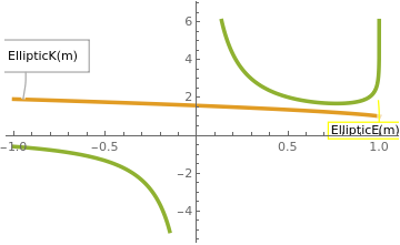
There are twelve Jacobi elliptic functions denoted by pq(x,m), where p and q are any of the letters c, s, n, and d. (Functions of the form pp(x,m) are trivially set to unity for notational completeness). The variable x is the argument, and m is the parameter, both of which may be complex. The first variable might be given in terms of the amplitude φ, or more commonly, in terms of x given below. The second variable might be given in terms of the parameter m, or as the elliptic modulus k, where k² = m, or in terms of the modular angle α, where m = sin²  α. The complements of k and m are defined as m' =1-m and \( k' = \sqrt {1-k^2} = \sqrt{1-m} . \) These four terms are used below without comment to simplify various expressions.

The elliptic sine sn x is given by

\[ \mbox{sn}(x,k) = \sin \varphi , \qquad x = \int_0^{\varphi} \frac{{\text d}\theta}{\sqrt{1 - k^2 \sin^2 \theta}} . \]
sn is pronounced roughly as “ess-en”. (Try saying three times fast: “ess-en u is the sine of the amplitude of u”). A plot of ()sn uvs. u looks very similar to a sine wave as seen in Figure

The elliptic cosine cn x is given by

\[ \mbox{cn}(x,k) = \cos \varphi , \qquad x = \int_0^{\varphi} \frac{{\text d}\theta}{\sqrt{1 - k^2 \sin^2 \theta}} . \]
The delta amplitude dn x is
\[ \mbox{dn}(x,k) = \sqrt{1 - k^2 \sin^2 \phi} . \]
Here, the angle φ is called the amplitude.

Some basic relations:

\begin{align*} \mbox{sn} (x,k) &= \frac{1}{\mbox{ns} (x,k)} , \qquad \mbox{cn} (x,k) = \frac{1}{\mbox{nc} (x,k)} , \qquad \mbox{dn} (x,k) = \frac{1}{\mbox{nd} (x,k)} , \\ \mbox{sd} (x,k) &= \frac{1}{\mbox{ds} (x,k)} , \qquad \mbox{cd} (x,k) = \frac{1}{\mbox{dc} (x,k)} , \qquad \mbox{sc} (x,k) = \frac{1}{\mbox{cs} (x,k)} . \end{align*}
Limiting values of k:

The Jacobi imaginary transformations relate various functions of the imaginary variable

\begin{align*} \mbox{cn} (x,k) &= \mbox{nc} ({\bf j}x,\sqrt{1-k^2}) , \qquad \mbox{cn} ({\bf j}x,k) = \mbox{nc} (x,\sqrt{1-k^2}) , \\ \mbox{sn} ({\bf j}x,k) &= {\bf j}\,\mbox{sc} ({\bf j}x,\sqrt{1-k^2}) , \qquad \mbox{sn} (x,k) = -{\bf j}\,\mbox{sc} ({\bf j}x,\sqrt{1-k^2}) , \\ \mbox{dn} ({\bf j}x,k) &= \mbox{dc} ({\bf j}x,\sqrt{1-k^2}) , \qquad \mbox{dn} (x,k) = \mbox{dc} ({\bf j}x,\sqrt{1-k^2}) . \end{align*}
First order derivatives:
\begin{align*} \frac{{\text d}}{{\text d} x}\, \mbox{sn}(x,k) &= \mbox{cn}(x,k) \, \mbox{dn}(x,k) , \\ \frac{{\text d}}{{\text d} x}\, \mbox{cn}(x,k) &= -\mbox{sn}(x,k) \, \mbox{dn}(x,k) , \\ \frac{{\text d}}{{\text d} x}\, \mbox{dn}(x,k) &= - k^2 \mbox{sn}(x,k) \, \mbox{cn}(x,k) , \\ \frac{{\text d}}{{\text d} x}\, \mbox{dc}(x,k) &= \left( 1 - k^2 \right) \mbox{sc}(x,k) \, \mbox{nc}(x,k) , \\ \frac{{\text d}}{{\text d} x}\, \mbox{nc}(x,k) &= \mbox{sc}(x,k) \, \mbox{nc}(x,k) , \\ \frac{{\text d}}{{\text d} x}\, \mbox{cd}(x,k) &= - \left( 1 - k^2 \right) \mbox{sd}(x,k) \, \mbox{nd}(x,k) , \\ \frac{{\text d}}{{\text d} x}\, \mbox{sd}(x,k) &= \mbox{cd}(x,k) \, \mbox{nd}(x,k) , \\ \frac{{\text d}}{{\text d} x}\, \mbox{ds}(x,k) &= -\mbox{cs}(x,k) \, \mbox{ns}(x,k) . \\ \end{align*}
Second order differential equations:
\begin{align*} \frac{{\text d}^2}{{\text d} x^2}\, \mbox{sn}(x,k) &= - \left( 1 + k^2 \right) \mbox{sn}(x,k) + 2k^2 \mbox{sn}^3 (x,k) , \\ \frac{{\text d}^2}{{\text d} x^2}\, \mbox{cn}(x,k) &= - \left( 1 -2 k^2 \right) \mbox{cn}(x,k) - 2k^2 \mbox{sn}^3 (x,k) , \\ \frac{{\text d}^2}{{\text d} x^2}\, \mbox{dn}(x,k) &= \left( 2- k^2 \right) \mbox{dn}(x,k) - 2\, \mbox{dn}^3 (x,k) , \\ \frac{{\text d}^2}{{\text d} x^2}\, \mbox{cd}(x,k) &= - \left( 1 + k^2 \right) \mbox{cd}(x,k) + 2k^2 \mbox{cd}^3 (x,k) , \\ \frac{{\text d}^2}{{\text d} x^2}\, \mbox{sd}(x,k) &= \left( 2 k^2 -1 \right) \mbox{sd}(x,k) - 2k^2 \left( 1 - k^2 \right) \mbox{sd}^3 (x,k) , \\ \frac{{\text d}^2}{{\text d} x^2}\, \mbox{nd}(x,k) &= \left( 2- k^2 \right) \mbox{nd}(x,k) - 2\left( 1 - k^2 \right) \mbox{dn}^3 (x,k) , \\ \frac{{\text d}^2}{{\text d} x^2}\, \mbox{dc}(x,k) &= - \left( 1 + k^2 \right) \mbox{dc}(x,k) + 2\, \mbox{dc}^3 (x,k) , \\ \frac{{\text d}^2}{{\text d} x^2}\, \mbox{nc}(x,k) &= - \left( 2k^2 -1 \right) \mbox{nc}(x,k) + 2\left( 1 - k^2 \right) \mbox{nc}^3 (x,k) , \\ \frac{{\text d}^2}{{\text d} x^2}\, \mbox{sc}(x,k) &= \left( 2 -k^2 \right) \mbox{sc}(x,k) + 2\left( 1 - k^2 \right) \mbox{sc}^3 (x,k) , \\ \frac{{\text d}^2}{{\text d} x^2}\, \mbox{ns}(x,k) &= -\left( 1+k^2 \right) \mbox{ns}(x,k) + 2\, \mbox{ns}^3 (x,k) , \\ \frac{{\text d}^2}{{\text d} x^2}\, \mbox{ds}(x,k) &= \left( 2k^2 -1 \right) \mbox{ds}(x,k) + 2\, \mbox{ds}^3 (x,k) , \\ \frac{{\text d}^2}{{\text d} x^2}\, \mbox{cs}(x,k) &= \left( 2 -k^2 \right) \mbox{cs}(x,k) + 2\, \mbox{cs}^3 (x,k) . \end{align*}

Airy functions are solutions to the Airy differential equation
y''[x] - x y[x] == 0
There are two linearly independent solutions, called by Mathematica as
AiryAi[x] and AiryBi[x].

Series[AiryAi[x], {x, 0, 9}]:
N[%]
Out[2]= 0.355028 -0.258819 x + 0.0591713 x^3 - 0.0215683 x^4 +
0.00197238 x^6 - 0.000513531 x^7 + 0.0000273941 x^9 - 5.7059 x
10^^{-6} + )(x)^10

Example: Consider an equation of ellipse written in the parametric form:

\[ \begin{split} x &= a\,\sin \phi , \\ y &= b\,\cos\phi , \end{split} \]
with 𝑎 > b. Its arclength s is
\[ s = a \int_0^{\phi} \sqrt{1 - k^2 \sin^2 \theta}\,{\text d}\theta \qquad \left( 0 \le \phi \le \frac{\pi}{2} \right) . \]
Then its length is expressed through the elliptic integral:
\[ \frac{s}{a} = E(\phi , k) , \qquad k^2 = 1 - \frac{b^2}{a^2} . \]
The total length of the ellipse is
\[ L(a,b) = 4a\, E(k) . \]
   ▣

Example: 
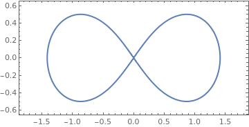
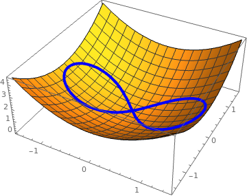
Lemniscate of Bernoulli is a special case of Cassinian oval. That is, the locus of points P, such that distance[P,F1] * distance[P,F2] == (distance[F1,F2]/2)^2, where F1, F2 are fixed points called foci. It is analogous to the definition of ellipse, where sum of two distances is replace by product.

Mathematica Notebook for This Page

The Bernoulli’s lemniscate is the inverse curve of an equilateral hyperbola:
\[ r^2 = 2a^2 \cos \left( 2 \theta \right) , \qquad 0 \le \theta \le \frac{\pi}{4} . \]
      We plot Bernoulli’s lemniscate with Mathematica:
ContourPlot[(x^2 + y^2)^2 == 2*(x^2 - y^2), {x, -1.8, 1.8}, {y, -0.63, 0.63}, ContourStyle -> Thick, AspectRatio -> 1/2]
       The Bernoulli’s lemniscate.            Mathematica code

      We plot Bernoulli’s lemniscate on the following surface
Plot3D[x^2 + y^2, {x, -1.2, 1.2}, {y, -1.2, 1.2}]
The following code allows you to visualize:
lem[t_] = TrigExpand[Sqrt[2] #/(#.#) &[{Sec[t], Tan[t]}]];
Show[Plot3D[x^2 + y^2, {x, -3/2, 3/2}, {y, -3/2, 3/2}], ParametricPlot3D[ Append[lem[t], Function[{x, y}, x^2 + y^2] @@ lem[t]], {t, 0, 2 \[Pi]}, PlotStyle -> {AbsoluteThickness[4], Blue}]]
       The Bernoulli’s lemniscate on the surface.            Mathematica code

You can achive the same graph using ContourPlot[]. Then you extract the Line[] objects and manipulate them like so:
lem = Cases[ Normal[ContourPlot[(x^2 + y^2)^2 == 2*(x^2 - y^2), {x, -1.8, 1.8}, {y, -0.63, 0.63}]], Line[l_] :> Line[Append[#, Function[{x, y}, x^2 + y^2] @@ #] & /@ l], \[Infinity]];
Show[Plot3D[x^2 + y^2, {x, -3/2, 3/2}, {y, -3/2, 3/2}], Graphics3D[{Directive[AbsoluteThickness[4], Blue], lem}]]
      You can make a fancy plot:
l[s_] := {(4 + 3 Sqrt[2] + (4 - 3 Sqrt[2]) s^4)/(3 + 2 Sqrt[2] + 6 s^2 + (3 - 2 Sqrt[2]) s^4), Sqrt[2] s (1/(1 + s^2) + 1/(-3 - 2 Sqrt[2] + (-3 + 2 Sqrt[2]) s^2))};
lp[s_] := Join[l[s], {0}];
f[s_] := Module[{p = l[s]}, {#1, #2, #1^2 + #2^2} & @@ p];
Show[ParametricPlot3D[{f[t], lp[t]}, {t, -400, 400}, PlotPoints -> 100, PlotRange -> {{-2.6, 2.6}, {-2.6, 2.6}, {0, 3}}, PlotStyle -> Red], Plot3D[x^2 + y^2, {x, -2.6, 2.6}, {y, -2.6, 2.6}, Mesh -> None, PlotStyle -> Opacity[0.5]], Background -> Black]
       The Bernoulli’s lemniscate on the surface.            Mathematica code

The arclength s of Bernoulli’s lemniscate is
\[ s = 2 a^2 \int_0^r \frac{{\text d}t}{\sqrt{4 a^4 - t^4}} = a\,F \left( \phi, 1/\sqrt{2} \right) \]
The perimeter length P of the lemniscate is given by
\[ P = 4a\,K\left( 1/\sqrt{2} \right) s = 2 a^2 \int_0^r \frac{{\text d}t}{\sqrt{4 a^4 - t^4}} = a\,F \left( \phi, 1/\sqrt{2} \right) = 2a\,\sqrt{2} \int_{-1}^1 \frac{{\text d}t}{\sqrt{1 - t^4}} = 4a\sqrt{2} F(1) = a\,\frac{\Gamma^2 (1/4)}{\sqrt{\pi}} \approx 7.416 \cdot a, \]
where F(x) is the elliptic integral
\[ F(x) = \int_0^x \frac{{\text d}t}{\sqrt{1 - t^4}} . \]
   ▣


Weierstrass elliptic functions


The principal difference between the Jacobiand the Weierstrass elliptic integrals is in the number of poles in each fundamentalcell. While the Jacobi elliptic functions has two simple poles per cell and can beconsiders as a solution to the differential equation
\[ \frac{{\text d}^2 x}{{\text d} t^2} = a + b\,x + c\,x^2 + d\,x^3 , \]
the Weierstrass elliptic functions have just one double pole and is a solution to
\[ \frac{{\text d}^2 x}{{\text d} t^2} = a + b\,x + c\,x^2 . \]


Theta Functions


Theta functions are the elliptic analogs of the exponential function and are typically written as θ𝑎(u, q), where 𝑎 ranges from 1 to 4 to represent the fours variations of the theta function, u is the argument of the function and q is the Nome, given as
\[ q = e^{{\bf j}\pi t} = e^{\pi\, K' /K} , \]
where
\[ t = - {\bf j}\, \frac{K' (k)}{K(k)} . \]

Example:    ▣


  1. Armitage, J. V. and Eberlein, W. F., Elliptic Functions, Cambridge University Press, 2006
  2. Filipuk, G., Introduction to elliptic functions,
  3. Finn, J.M., Introduction to the Special Functions of Mathematical Physics with applications to the physical and applied sciences, 2005.
  4. Prasolov, V. and Solovyev, Y.,Elliptic Functions and Elliptic Integrals, Amer.Math. Soc., Providence, RI, 1997.
  5. Trachev, V.G., Elliptic functions: Introductory course, 2005.
  6. Weisstein, E.W., Books about Elliptic Integrals, http://www.ericweisstein.com/encyclopedias/books/EllipticIntegrals.html.
  7. Whittaker, E.T. and Watson, G.N. A Course in Modern Analysis, 4th ed., Cam-bridge University Press, Cambridge, England, 1990.


Return to Mathematica page)
Return to the main page (APMA0340)
Return to the Part 1 Matrix Algebra
Return to the Part 2 Linear Systems of Ordinary Differential Equations
Return to the Part 3 Non-linear Systems of Ordinary Differential Equations
Return to the Part 4 Numerical Methods
Return to the Part 5 Fourier Series
Return to the Part 6 Partial Differential Equations
Return to the Part 7 Special Functions