Preface


This section presents a remarkable formula, discovered by James Sylvester in 1883, used for defining a function of a square matrix. The beauty of this formula is based on generalization of the Lagrange interpolation polynomials for matrices that are now called Sylvester's auxiliary matrices. The Sylvester formula provides an efficient way to represent a function of a square diagonalizable matrix as a linear combination of auxiliary matrices. It turns out that these Sylvester's auxiliary matrices are projection matrices on eigenspaces for the given matrix. Although the Sylvester formula is applicable only for diagonalizable matrices, it has an extension due to Arthur Buchheim (1886) that covers the general case, but it loses its beauty and simplicity.

Return to computing page for the first course APMA0330
Return to computing page for the second course APMA0340
Return to Mathematica tutorial for the first course APMA0330
Return to Mathematica tutorial for the second course APMA0340
Return to the main page for the first course APMA0330
Return to the main page for the second course APMA0340
Return to Part I of the course APMA0340
Introduction to Linear Algebra with Mathematica

Sylvester Formula


 To understand the Sylvester formula, we need to introduce some important definitions and statements, including the famous Cayley--Hamilton theorem. Since our objective is to define a function of a square matrix, it makes sense to start with the simplest class of functions---a set of polynomials. We single out polynomials because for each such function \( q \left( \lambda \right) = q_0 + q_1 \lambda + q_2 \lambda^2 + \cdots + q_n \lambda^n \) we can naturally assign a matrix \( q \left( {\bf A} \right) = q_0 {\bf I} + q_1 {\bf A} + q_2 {\bf A}^2 + \cdots + q_n {\bf A}^n . \) It is obvious that multiplication of square matrices and their addition/subtraction is well defined and understood.

A scalar polynomial \( q \left( \lambda \right) \) is called an annulled polynomial (or annihilating polynomial) of the square matrix A, if \( q \left( {\bf A} \right) = {\bf 0} , \) with the understanding that \( {\bf A}^0 = {\bf I} , \) the identity matrix, replaces \( \lambda^0 =1 \) when substituting A for λ.
The minimal polynomial of a square matrix A is a unique monic polynomial ψ of lowest degree such that \( \psi \left( {\bf A} \right) = {\bf 0} . \) Every square matrix has a minimal polynomial.
A square matrix A for which the characteristic polynomial \( \chi (\lambda ) = \det \left( \lambda {\bf I} - {\bf A} \right) \) and the minimal polynomial are the same is called a nonderogatory matrix (where I is the identity matrix). A derogatory matrix is one where the characteristic polynomial and minimal polynomial are not the same.
A n×n matrix with n distinct eigenvalues is a nonderogatory matrix. However, if a diagonalizable matrix A has multiple eigenvalues (they are multiple roots of the algebraic equation det(λIA) = 0) in λ), it is derogatory.
Example 1: Consider two matrices
\[ {\bf A} = \begin{bmatrix} 11&-4&-2 \\ 20&-7&-4 \\ \phantom{1}5&-2&\phantom{-}0 \end{bmatrix} \qquad\mbox{and} \qquad {\bf B} = \begin{bmatrix} 13&-5&-2 \\ 24&-9&-4 \\ \phantom{1}7&-3&\phantom{-}0 \end{bmatrix} \]
that share the same characteristic polynomial:
\begin{align*} \chi_{\bf A} (\lambda ) &= \det \left( \lambda {\bf I} - {\bf A} \right) = \det \left( \lambda \begin{bmatrix} 1&0&0 \\ 0&1&0 \\ 0&0&1 \end{bmatrix} - \begin{bmatrix} 11&-4&-2 \\ 20&-7&-4 \\ \phantom{1}5&-2& \phantom{-}0 \end{bmatrix} \right) = \det \begin{bmatrix} \lambda -11&4&2 \\ -20&\lambda +7&4 \\ -5&2&\lambda \end{bmatrix} = \lambda^3 - 4\,\lambda^2 + 5\,\lambda -2 , \\ \chi_{\bf B} (\lambda ) &= \det \left( \lambda {\bf I} - {\bf B} \right) = \chi_{\bf B} (\lambda ) = \left( \lambda -1 \right)^2 (\lambda -2) = \lambda^3 - 4\,\lambda^2 + 5\,\lambda -2 . \end{align*}
A = {{11,-4,-2}, {20,-7,-4}, {5,-2,0}}
B = {{13,-5,-2}, {24,-9,-4}, {7,-3,0}}
CharacteristicPolynomial[A,lambda]
Factor[%]
Det[lambda*IdentityMatrix[3]-B]
Factor[%]
We show that matrix A is annihilated by the characteristic polynomial:
\begin{align*} {\bf A}^3 -4\,{\bf A}^2 + 5\,{\bf A} -2\,{\bf A}^0 &= \begin{bmatrix} \phantom{1}71&-28&-14 \\ 140&-55&-28 \\ \phantom{1}35&-14&-6\phantom{1} \end{bmatrix} -4 \begin{bmatrix} 31&-12&\phantom{1}-6 \\ 60&-23&-12 \\ 15&-6&-2 \end{bmatrix} + 5 \begin{bmatrix} 11&-4&-2 \\ 20&-7&-4 \\ \phantom{1}5&-2&\phantom{-}0 \end{bmatrix} -2 \begin{bmatrix} 1&0&0 \\ 0&1&0 \\ 0&0&1 \end{bmatrix} \\ &= \begin{bmatrix} 0&0&0 \\ 0&0&0 \\ 0&0&0 \end{bmatrix} \end{align*}
and similarly for matrix B
\begin{align*} {\bf B}^3 -4\,{\bf B}^2 + 5\,{\bf B} -2\,{\bf B}^0 &= \begin{bmatrix} \phantom{1}77&-31&-14 \\ 152&-61&-28 \\ \phantom{1}41&-17&\phantom{1}-6 \end{bmatrix} -4 \begin{bmatrix} 35&-14&-6 \\ 68&-27&-12 \\ 19&-8&-2 \end{bmatrix} + 5 \begin{bmatrix} 13&-5&-2 \\ 24&-9&-4 \\ -7&-3&\phantom{-}0 \end{bmatrix} -2 \begin{bmatrix} 1&0&0 \\ 0&1&0 \\ 0&0&1 \end{bmatrix} \\ & = \begin{bmatrix} 0&0&0 \\ 0&0&0 \\ 0&0&0 \end{bmatrix} . \end{align*}
On the other hand, the minimal polynomial for matrix A is
\[ \psi_{\bf A} (\lambda ) = \left( \lambda -1 \right) \left( \lambda -2 \right) = \lambda^2 -3\,\lambda +2 \]
since
\begin{align*} \psi_{\bf A} \left({\bf A} \right) &= \left( {\bf A} - {\bf I} \right) \left( {\bf A} -2 {\bf I} \right) = {\bf A}^2 -3\,{\bf A} +2 \,{\bf I} \\ &= \begin{bmatrix} 31&-12&-6 \\ 60&-23&-12 \\ 15&-6&-2 \end{bmatrix} - 3 \begin{bmatrix} 11&-4&-2 \\ 20&-7&-4 \\ 5&-2&0 \end{bmatrix} +2 \begin{bmatrix} 1&0&0 \\ 0&1&0 \\ 0&0&1 \end{bmatrix} = \begin{bmatrix} 0&0&0 \\ 0&0&0 \\ 0&0&0 \end{bmatrix} . \end{align*}
Therefore, matrix A is a derogatory matrix. However, matrix B is a nonderogatory matrix because
\[ \psi_{\bf B} (\lambda ) = \left( \lambda -1 \right)^2 \left( \lambda -2 \right) = \lambda^3 - 4\,\lambda^2 +5\,\lambda -2 = \chi_B (\lambda ) . \qquad\quad ■ \]
Example 2: Consider the matrix
\[ {\bf T} = \begin{bmatrix} 29&390&336&648&-480 \\ 3&26&24 & 48&-36 \\ 12&153&131&255&-189 \\ 6&69&60&116&-87 \\ 21&249&216&420&-313 \end{bmatrix} . \]
Its characteristic polynomial is of degree 5:
T = {{29,390,336,648,-480}, {3,26,24,48,-36}, {12,153,131,255,-189}, {6,69,60,116,-87}, {21,249,216,420,-313}}
Det[s*IdentityMatrix[5] - T]
Factor[%]
\[ \chi \left( \lambda \right) = \det \left( \lambda {\bf I} - {\bf A} \right) = \left( \lambda +1 \right)^3 \left( \lambda +4 \right)^2 = \lambda^5 +11\,\lambda^4 + 43\,\lambda^3 + 73\,\lambda^2 + 58\,\lambda +16 ; \]
however, its minimal polynomial is of degree 2:
\[ \psi \left( \lambda \right) = \left( \lambda +1 \right) \left( \lambda +4 \right) = \lambda^2 + 5\,\lambda + 4 . \]
Indeed,
\begin{align*} \psi \left( {\bf T} \right) &= \left( {\bf T} +{\bf I} \right) \left( {\bf T} +4\,{\bf I} \right) = {\bf T}^2 + 5\,{\bf T} + 4\,{\bf I} \\ &= \begin{bmatrix} -149&-1950&-1680&-3240&2400 \\ -15&-134&-120 &-240&180 \\ -60&-765&-659&-1275&945 \\ -30&-345&-300&-584&435 \\ -105&-1245&-1080&-2100&1561 \end{bmatrix} +5 \begin{bmatrix} 29&390&336&648&-480 \\ 3&26&24 & 48&-36 \\ 12&153&131&255&-189 \\ 6&69&60&116&-87 \\ 21&249&216&420&-313 \end{bmatrix} + 4 \begin{bmatrix} 1&0&0&0&0 \\ 0&1&0 &0&0 \\ 0&0&1&0&0 \\ 0&0&0&1&0 \\ 0&0&0&0&1 \end{bmatrix} \\ &= \begin{bmatrix} 0&0&0&0&0 \\ 0&0&0&0&0 \\ 0&0&0&0&0 \\ 0&0&0&0&0 \\ 0&0&0&0&0 \end{bmatrix} . \end{align*}
Therefore, matrix T is a derogatory matrix.   ■

         
     Arthur Cayley        James Sylvester        William Hamilton
Theorem: (Cayley--Hamilton) Every square matrix A is annulled by its characteristic polynomial, that is, \( \chi ({\bf A}) = {\bf 0} , \) where \( \chi (\lambda ) = \det \left( \lambda {\bf I} - {\bf A} \right) . \)  ▣
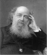
Arthur Cayley (1821--1895) was a British mathematician, and a founder of the modern British school of pure mathematics. As a child, Cayley enjoyed solving complex math problems for amusement. He entered Trinity College, Cambridge, where he excelled in Greek, French, German, and Italian, as well as mathematics. He worked as a lawyer for 14 years. During this period of his life, Cayley produced between two and three hundred mathematical papers. Many of his publications were results of collaboration with his friend J. J. Sylvester.

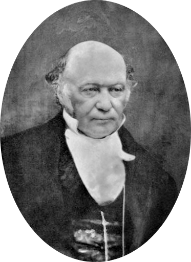
Sir William Rowan Hamilton (1805--1865) was an Irish physicist, astronomer, and mathematician, who made important contributions to classical mechanics, optics, and algebra. He was the first foreign member of the American National Academy of Sciences. Hamilton had a remarkable ability to learn languages, including modern European languages, Hebrew, Persian, Arabic, Hindustani, Sanskrit, and even Marathi and Malay. Hamilton was part of a small but well-regarded school of mathematicians associated with Trinity College in Dublin, which he entered at age 18. Strangely, the credit for discovering the quantity now called the Lagrangian and Lagrange's equations belongs to Hamilton. In 1835, being secretary to the meeting of the British Science Association which was held that year in Dublin, he was knighted by the lord-lieutenant.

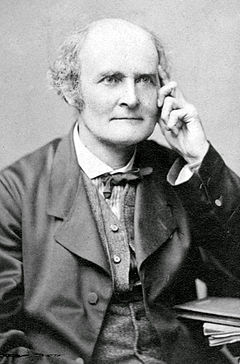
James Joseph Sylvester (1814--1897) was an English mathematician. He made fundamental contributions to matrix theory, invariant theory, number theory, partition theory, and combinatorics. Sylvester was born James Joseph in London, England, but later, when his older brother changed it to "Sylvester" upon emigration to the United States, James followed suit. At the age of 14, Sylvester was a student of Augustus De Morgan at the University of London. His family withdrew him from the University after he was accused of stabbing a fellow student with a knife. Subsequently, he attended the Liverpool Royal Institution.

However, Sylvester was not issued a degree, because graduates at that time were required to state their acceptance of the Thirty-Nine Articles of the Church of England, and Sylvester could not do so because he was Jewish. The same reason was given in 1843 for his being denied appointment as Professor of Mathematics at Columbia College (now University) in New York City. After, for the same reason, he was unable to compete for a Fellowship or obtain a Smith's prize. In 1838 Sylvester became professor of natural philosophy at University College London and in 1839 a Fellow of the Royal Society of London. In 1841, he was awarded a BA and an MA by Trinity College, Dublin. In the same year he moved to the United States to become a professor of mathematics at the University of Virginia, but left after less than four months following a violent encounter with two students he had disciplined. He moved to New York City and began friendships with the Harvard mathematician Benjamin Peirce and the Princeton physicist Joseph Henry, but in November 1843, after his rejection by Columbia, he returned to England.

For long period of time, 1843--1855, James Sylvester supported his living by developing actuarial models, practicing law and being a music tutor.

One of Sylvester's lifelong passions was for poetry; he read and translated works from the original French, German, Italian, Latin and Greek, and many of his mathematical papers contain illustrative quotes from classical poetry. In 1876, Sylvester again crossed the Atlantic Ocean to become the inaugural professor of mathematics at the new Johns Hopkins University in Baltimore, Maryland. His salary was $5,000 (quite generous for the time), which he demanded be paid in gold. After negotiation, an agreement was reached on a salary that was not paid in gold. In 1878, he founded the American Journal of Mathematics. In 1883, he returned to England to take up the Savilian Professor of Geometry at Oxford University. He held this chair until his death. Sylvester invented a great number of mathematical terms such as "matrix" (in 1850), "graph" (combinatorics) and "discriminant." He coined the term "totient" for Euler's totient function.

Privately, Sylvester suffered from depression for almost three years, during which he completed no mathematical research but then Pafnuty Chebyshev visited London and the two discussed mechanical linkages which can be used to draw straight lines. After working on this topic, Sylvester began giving an evening lecture titled "On recent discoveries in mechanical conversion of motion" at the Royal Institution. One mathematician in the audience at this lecture was Alfred Kempe and he became absorbed by this topic. Kempe and Sylvester worked jointly on linkages and made important discoveries.    ✶

Theorem 2: For polynomials p and q and a square matrix A, \( p \left( {\bf A} \right) = q \left( {\bf A} \right) \) if and only if p and q take the same values on the spectrum (set of all eigenvalues) of A.
Theorem 3: The minimal polynomial ψ of a square matrix A divides any other annihilating polynomial p for which \( p \left( {\bf A} \right) = {\bf 0} . \) In particular, the minimal polynomial divides the characteristic polynomial of A.  ▣

 From Theorem 3, it follows that the minimal polynomial is always a product of monomials \( \lambda - \lambda_i \) for each eigenvalue λi because the characteristic polynomial contains all such multiples. So all eigenvalues must be present in the product form for a minimal polynomial.

Theorem 4: The minimal polynomial for a linear operator on a finite-dimensional vector space is unique.
Theorem 5: A square n×n matrix A is diagonalizable if and only if its minimal polynomial is a product of simple terms: \( \psi (\lambda ) = \left( \lambda - \lambda_1 \right) \left( \lambda - \lambda_2 \right) \cdots \left( \lambda - \lambda_r \right) , \) where λ1, … , λr are the distinct eigenvalues of matrix A (rn).

  Therefore, a square matrix A is not diagonalizable if and only if its minimal polynomial contains at least one multiple \( \left( \lambda - \lambda_1 \right)^m \) for m > 1.

Theorem 6: Every matrix that commutes with a square matrix A is a polynomial in A if and only if A is nonderogatory.
Theorem 7: If A is upper triangular and nonderogatory, then any solution X of the equation \( f \left( {\bf X} \right) = {\bf A} \) is upper triangular.  ▣

 In Mathematica, one can define the minimal polynomial using the following code:

MatrixMinimalPolynomial[a_List?MatrixQ, x_] :=
Module[{i, n = 1, qu = {},
mnm = {Flatten[IdentityMatrix[Length[a]]]}},
While[Length[qu] == 0, AppendTo[mnm, Flatten[MatrixPower[a, n]]];
qu = NullSpace[Transpose[mnm]];
n++];
First[qu].Table[x^i, {i, 0, n - 1}]]
Then to find a minimal polynomial of previously defined square matrix A, just enter
MatrixMinimalPolynomial[A, x]

Suppose that A is a diagonalizable n×n matrix; this means that all its eigenvalues are not defective and there exists a basis of n linearly independent eigenvectors. Then its minimal polynomial (the polynomial of least possible degree that annihilates the matrix) is a product of simple terms:

\begin{equation} \label{EqSylvester.1} \psi (\lambda ) = \left( \lambda - \lambda_1 \right) \left( \lambda - \lambda_2 \right) \cdots \left( \lambda - \lambda_k \right) , \end{equation}
where \( \lambda_1 , \lambda_2 , \ldots , \lambda_k \) are distinct eigenvalues of matrix A ( \( k \le n \) ).

Let \( f(\lambda ) \) be a function defined on the spectrum of the matrix A. We assume that every eigenvalue λi is in the domain of f, and that every eigenvalue λi with multiplicity mi > 1 is in the interior of the domain, with f being (mi — 1) times differentiable at λi. We build a function \( f\left( {\bf A} \right) \) of diagonalizable square matrix A according to James Sylvester, who was an English lawyer and music tutor before his appointment as a professor of mathematics in 1885. To define a function of a square matrix, we need to construct k Sylvester auxiliary matrices for each distinct eigenvalue \( \lambda_i , \quad i= 1,2,\ldots k: \)

\begin{equation} \label{EqSylvester.2} {\bf Z}_{\lambda_i} = {\bf Z}_{i} = \dfrac{\left( {\bf A} - \lambda_1 {\bf I} \right) \cdots \left( {\bf A} - \lambda_{i-1} {\bf I} \right) \left( {\bf A} - \lambda_{i+1} {\bf I} \right) \cdots \left( {\bf A} - \lambda_k {\bf I} \right)}{(\lambda_i - \lambda_1 ) \cdots (\lambda_i - \lambda_{i-1} ) (\lambda_i - \lambda_{i+1} ) \cdots (\lambda_i - \lambda_k )} . \end{equation}
Sylvester's auxiliary matrix \( {\bf Z}_i \) is actually the Lagrange interpolating polynomial. The denominator in Eq.\eqref{EqSylvester.2} is actually the derivative of the minimal polynomial evaluated at λi:
\[ \psi' \left( \lambda_i \right) = (\lambda_i - \lambda_1 ) \cdots (\lambda_i - \lambda_{i-1} ) (\lambda_i - \lambda_{i+1} ) \cdots (\lambda_i - \lambda_k ) , \qquad i=1,2,\ldots , k . \]
Then Sylvester's auxiliary matrix can be written in a compact form:
\[ {\bf Z}_{\lambda_i} = \frac{\psi' \left( \lambda = \lambda_i = {\bf A} \right)}{\psi' \left( \lambda_i \right)} , \qquad i=1,2,\ldots , k . \]
Now we define the function \( f\left( {\bf A} \right) \) according to the formula:
\begin{equation} \label{EqSylvester.3} f\left( {\bf A} \right) = \sum_{i=1}^k f(\lambda_i )\,{\bf Z}_i . \end{equation}
Theorem 8: Each Sylvester's matrix \( {\bf Z}_i \) is a projection matrix on the eigenspace of the corresponding eigenvalue, so \( {\bf Z}_i^2 = {\bf Z}_i , \ i = 1,2,\ldots , r. \) Moreover, these auxiliary matrices are orthogonal, so \( {\bf Z}_i {\bf Z}_j = {\bf 0} \) for ij. A Sylvester's matrix \( {\bf Z}_i \) is an eigenmatrix corresponding to the eigenvalue λi:
\begin{equation} \label{EqSylvester.4} {\bf A} \,{\bf Z}_i = \lambda_i {\bf Z}_i , \qquad i=1,2,\ldots r. \end{equation}

In particular, we get from Sylvester's formula \eqref{EqSylvester.3} the spectral decomposition of a square diagonalizable matrix A:

\begin{equation} \label{EqSylvester.5} {\bf A} = \sum_{i=1}^k \lambda_i \,{\bf Z}_i . \end{equation}

Example 3: Consider a 2-by-2 matrix
\[ {\bf A} = \begin{bmatrix} \phantom{-}4&\phantom{-}5 \\ -1& -2 \end{bmatrix} \]
that has two distinct eigenvalues \( \lambda_1 =3 \) and \( \lambda_2 =-1 . \) The eigenvectors corresponding to these eigenvalues are
A = {{4, 5}, {-1, -2}}
Eigenvalues[A]
Eigenvectors[A]
\[ {\bf v}_1 = \left\langle -5 , \ 1 \right\rangle^{\mathrm T} \qquad {\bf v}_2 = \left\langle 1 , \ -1 \right\rangle^{\mathrm T} , \]

respectively. Here the superscript "T" represents transposition because it is a custom to use column vectors. Since the minimal polynomial is \( \psi (\lambda ) = (\lambda -3)(\lambda +1) \) is a product of simple factors, we build Sylvester's auxiliary matrices:
Zm1 = (A - 3*IdentityMatrix[2])/(-4)
Z3 = (A + IdentityMatrix[2])/4
\[ {\bf Z}_3 = \frac{{\bf A} +1}{3+1} = \frac{1}{4} \begin{bmatrix} \phantom{-}5 & \phantom{-}5 \\ -1& -1 \end{bmatrix} \quad\mbox{and} \quad {\bf Z}_{(-1)} = \frac{{\bf A} -3}{-1-3} = \frac{1}{4} \begin{bmatrix} -1&-5 \\ \phantom{-}1&\phantom{-}5 \end{bmatrix} . \]
These matrices are projectors on eigenspaces:
\[ {\bf Z}_3^2 = {\bf Z}_3 \qquad \mbox{and} \qquad {\bf Z}_{(-1)}^2 = {\bf Z}_{(-1)} , \quad \mbox{but} \quad {\bf Z}_3 {\bf Z}_{(-1)} = {\bf 0}. \]
Let us take an arbitrary vector, say \( {\bf x} = \langle 2, \ 2 \rangle^{\mathrm T} , \) and expand it with respect to eigenvectors:
\[ {\bf x} = \begin{bmatrix} 2 \\ 2 \end{bmatrix} = a\, {\bf v}_1 + b\,{\bf v}_2 = a \begin{bmatrix} -5 \\ \phantom{-}1 \end{bmatrix} + b \begin{bmatrix} \phantom{-}1 \\ -1 \end{bmatrix} , \]
where coefficients 𝑎 and b need to be determined. Of course, we can find them by solving the system of linear equations:
\[ \begin{split} 2 &= a(-5) + b , \\ 2 &= a - b . \end{split} \]
However, an easier way to do this is to apply Sylvester's auxiliary matrices:
\begin{align*} {\bf Z}_3 \, {\bf x} &= \frac{1}{4} \begin{bmatrix} \phantom{-}5& \phantom{-}5 \\ -1& -1 \end{bmatrix} \, \begin{bmatrix} 2\\ 2 \end{bmatrix} = \frac{1}{2} \begin{bmatrix} 5&5 \\ -1& -1 \end{bmatrix} \, \begin{bmatrix} 1 \\ 1 \end{bmatrix} = \frac{1}{2} \begin{bmatrix} 10 \\ 2 \end{bmatrix} = \begin{bmatrix} \phantom{-}5\\ -1 \end{bmatrix} = -{\bf v}_1 , \\ {\bf Z}_{(-1)}\, {\bf x} &= \frac{1}{4} \begin{bmatrix} -1&-5 \\ \phantom{-}1 &\phantom{-}5 \end{bmatrix} \, \begin{bmatrix} 2\\ 2 \end{bmatrix} = \begin{bmatrix} -3 \\ \phantom{-}3 \end{bmatrix} = -3\, {\bf v}_2 . \end{align*}
Therefore, coefficients are \( a =-1 \) and \( b =-3 . \) So we get the expansion:
\[ {\bf x} = \begin{bmatrix} 2 \\ 2 \end{bmatrix} = - {\bf v}_1 - 3\,{\bf v}_2 = - \begin{bmatrix} -5 \\ \phantom{-}1 \end{bmatrix} -3 \begin{bmatrix} \phantom{-}1 \\ -1 \end{bmatrix} . \]
Illustrating Eq.\eqref{EqSylvester.3} with functions f(λ) defined on the spectrum of matrix A, we consider \( U(\lambda ) = e^{\lambda \,t} \) and \( \psi (\lambda ) = \cos \left( \lambda \,t\right) , \) which are functions of a variable λ depending on a real parameter t that is usually associated with time. Indeed,
\begin{align*} U({\bf A}) &= e^{3t}\, {\bf Z}_3 + e^{-t}\, {\bf Z}_{(-1)} = e^{3t}\, \frac{1}{4} \begin{bmatrix} \phantom{-}5&\phantom{-}5 \\ -1& -1 \end{bmatrix} + e^{-t} \, \frac{1}{4} \begin{bmatrix} -1&-5 \\ \phantom{-}1\phantom{-}&5 \end{bmatrix} , \\ \psi ({\bf A}) &= \cos (3t) \, {\bf Z}_3 + \cos\, t\, {\bf Z}_{(-1)} = \frac{\cos \,3t}{4} \begin{bmatrix} 5&5 \\ -1& -1 \end{bmatrix} + \frac{\cos\, t}{4} \begin{bmatrix} -1&-5 \\ 1&5 \end{bmatrix} .\end{align*}
Example 4: Consider the \( 3 \times 3 \) matrix \( {\bf A} = \begin{bmatrix} \phantom{-}1&\phantom{-}4&16 \\ \phantom{-}18& \phantom{-}20&\phantom{-}4 \\ -12&-14&-7 \end{bmatrix} \) that has three distinct eigenvalues; Mathematica confirms
A = {{1,4,16},{18,20,4},{-12,-14,-7}}
Eigenvalues[A]
Out[2]= 9, 4, 1
Then we define Sylvester auxiliary matrices
\[ {\bf Z}_1 = \frac{\left( {\bf A} - 9{\bf I} \right)\left( {\bf A} - 4{\bf I} \right)}{(1-9)(1-4)} = \begin{bmatrix} -4&-8&-12 \\ \phantom{-}4& \phantom{-}8&\phantom{-}12 \\ -1&-2&-3 \end{bmatrix}, \quad {\bf Z}_4 = \frac{\left( {\bf A} - 9{\bf I} \right)\left( {\bf A} - {\bf I} \right)}{(4-9)(4-1)} = \begin{bmatrix} \phantom{-}8&\phantom{-}12& \phantom{-}16 \\ -10&-15&-20 \\ \phantom{-}4& \phantom{-}6&\phantom{-}8 \end{bmatrix} , \quad {\bf Z}_9 = \frac{\left( {\bf A} - 4{\bf I} \right)\left( {\bf A} - {\bf I} \right)}{(9-1)(9-4)} = \begin{bmatrix} -3&-4&-4 \\ \phantom{-}6& \phantom{-}8& \phantom{-}8 \\ -3&-4&-4 \end{bmatrix} . \]
We check with Mathematica that these auxiliary matrices are projectors:
Z1 = (A - 9*IdentityMatrix[3]).(A - 4*IdentityMatrix[3])/3/8
{{-4, -8, -12}, {4, 8, 12}, {-1, -2, -3}}
Z4 = (A - 9*IdentityMatrix[3]).(A - 1*IdentityMatrix[3])/(4 - 9)/(4 - 1)
{{8, 12, 16}, {-10, -15, -20}, {4, 6, 8}}
Z9 = (A - 4*IdentityMatrix[3]).(A - 1*IdentityMatrix[3])/(9 - 4)/(9 - 1)
{{-3, -4, -4}, {6, 8, 8}, {-3, -4, -4}}
Eigenvalues[Z1]
{1, 0, 0}
Eigenvectors[Z1]
{{4, -4, 1}, {-3, 0, 1}, {-2, 1, 0}}
Eigenvalues[Z4]
{1, 0, 0}
Eigenvectors[Z4]
{{4, -5, 2}, {-2, 0, 1}, {-3, 2, 0}}
Eigenvalues[Z9]
{1, 0, 0}
Eigenvectors[Z9]
{{1, -2, 1}, {-4, 0, 3}, {-4, 3, 0}}
Now we demonstrate that these auxiliary matrices are mutually orthogonal by multiplying them to get a product to be zero.
Z1.Z4
{{0, 0, 0}, {0, 0, 0}, {0, 0, 0}}
Z1.Z1 - Z1
{{0, 0, 0}, {0, 0, 0}, {0, 0, 0}}
Z1.Z9
{{0, 0, 0}, {0, 0, 0}, {0, 0, 0}}
Z4.Z4 - Z4
{{0, 0, 0}, {0, 0, 0}, {0, 0, 0}}
Z9.Z4
{{0, 0, 0}, {0, 0, 0}, {0, 0, 0}}
Z9.Z9 - Z9
{{0, 0, 0}, {0, 0, 0}, {0, 0, 0}}

With Sylvester's matrices, we are able to construct arbitrary admissible functions of the given matrix. We start with the square root function \( r(\lambda ) = \sqrt{\lambda} , \) which is actually comprised of two branches \( r(\lambda ) = \sqrt{\lambda} \) and \( r(\lambda ) = -\sqrt{\lambda} . \) Indeed, choosing a particular branch, we get

\begin{align*} {\bf R}_1 &= {\bf Z}_1 + 2\,{\bf Z}_4 + 3\, {\bf Z}_9 = \begin{bmatrix} \phantom{-}3& \phantom{-}4& \phantom{-}8 \\ \phantom{-}2& \phantom{-}2&-4 \\ -2&-2&\phantom{-}1 \end{bmatrix} , \\ {\bf R}_2 &= {\bf Z}_1 - 2\,{\bf Z}_4 + 3\, {\bf Z}_9 = \begin{bmatrix} -29&-44&-56 \\ \phantom{-}42&\phantom{-}62&\phantom{-}76 \\ -18&-26&-31 \end{bmatrix} , \\ {\bf R}_3 &= {\bf Z}_1 + 2\,{\bf Z}_4 - 3\, {\bf Z}_9 = \begin{bmatrix} \phantom{-}21&\phantom{-}28&\phantom{-}32 \\ -34&-46&-52 \\ \phantom{-}16&\phantom{-}22&\phantom{-}25 \end{bmatrix} , \\ {\bf R}_4 &= {\bf Z}_1 - 2\,{\bf Z}_4 - 3\, {\bf Z}_9 = \begin{bmatrix} -11&-20&-32 \\ \phantom{-}6&\phantom{-}14&\phantom{-}28 \\ \phantom{-}0&-2&-7 \end{bmatrix} . \end{align*}
The other four roots are the negatives of these matrices.

We consider two other functions \( \displaystyle \Phi (\lambda ) = \frac{\sin \left( t\,\sqrt{\lambda} \right)}{\sqrt{\lambda}} \) and \( \displaystyle \Psi (\lambda ) = \cos \left( t\,\sqrt{\lambda} \right) . \) It is not a problem to determine the corresponding matrix functions

\begin{align*} {\bf \Phi} (t) &= \frac{\sin \left( \sqrt{\bf A}\,t \right)}{\sqrt{\bf A}} = \sin t \,{\bf Z}_1 + \frac{\sin 2\,t}{2} \,{\bf Z}_4 + \frac{\sin 3\,t}{3}\, {\bf Z}_9 , \\ {\bf \Psi} (t) &= \cos \left( \sqrt{\bf A}\,t \right) = \cos t\,{\bf Z}_1 + \cos 2\,t\,{\bf Z}_4 + \cos 3\,t\, {\bf Z}_9 . \end{align*}
These two matrix functions are solutions of the matrix differential equation \( \displaystyle \ddot{\bf P} (t) + {\bf A}\,{\bf P} (t) = {\bf 0} \) subject to the initial conditions
\[ {\bf \Phi} (0) = {\bf 0} , \quad \dot{\bf \Phi} (0) = {\bf I} , \quad {\bf \Psi} (0) = {\bf I} , \quad \dot{\bf \Psi} (0) = {\bf 0} \]
because \( \displaystyle {\bf Z}_1 + {\bf Z}_4 + {\bf Z}_9 = {\bf I} \) and \( \displaystyle {\bf A}\,{\bf Z}_1 - {\bf Z}_1 = {\bf 0}, \quad {\bf A}\,{\bf Z}_4 - 4\,{\bf Z}_4 = {\bf 0}, \quad {\bf A}\,{\bf Z}_9 - 9\,{\bf Z}_9 = {\bf 0} . \)
Example 5: Consider the nonderogatory (diagonalizable) \( 3 \times 3 \) matrix \( {\bf A} = \begin{bmatrix} -20&-42&-21 \\ \phantom{-}6& \phantom{-}13& \phantom{-}6 \\ \phantom{-}12&\phantom{-}24&\phantom{-}13 \end{bmatrix} \) that has only two \phantom{-}\phantom{-}\phantom{-}distinct eigenvalues
A = {{-20, -42, -21}, {6, 13, 6}, {12, 24, 13}};
Eigenvalues[A]
Out[2]= 4, 1, 1
We define the resolvent:
\[ {\bf R}_{\lambda} ({\bf A}) = \left( \lambda {\bf I} - {\bf A} \right)^{-1} = \frac{1}{(\lambda -1)(\lambda -4)} \,\begin{bmatrix} \lambda -25 & -42 & -21 \\ 6 & 8+\lambda & 6 \\ 12&24&8+\lambda \end{bmatrix} . \]
to verify that the minimal polynomial is a product of simple terms. Recall that the denominator in a resolvent (upon reducing all common multiples) is always the minimal polynomial.
resolvent = FullSimplify[Inverse[lambda*IdentityMatrix[3] - A]]
Out[2]= {{(-25 + lambda)/( 4 - 5 lambda + lambda^2), -(42/(4 - 5 lambda + lambda^2)), -(21/( 4 - 5 lambda + lambda^2))}, {6/(4 - 5 lambda + lambda^2), ( 8 + lambda)/(4 - 5 lambda + lambda^2), 6/( 4 - 5 lambda + lambda^2)}, {12/(4 - 5 lambda + lambda^2), 24/( 4 - 5 lambda + lambda^2), (8 + lambda)/(4 - 5 lambda + lambda^2)}}
Using the resolvent, we define Sylvester's auxiliary matrices:
Z1 = FullSimplify[(lambda - 1)*resolvent] /. lambda -> 1
Out[3]= {{8, 14, 7}, {-2, -3, -2}, {-4, -8, -3}}
Z4 = FullSimplify[(lambda - 4)*resolvent] /. lambda -> 4
Out[4]= {{-7, -14, -7}, {2, 4, 2}, {4, 8, 4}}
\[ {\bf Z}_1 = \begin{bmatrix} \phantom{-}8&14&\phantom{-}7 \\ -2& -3&-2 \\ -4&-8&-3 \end{bmatrix} , \qquad {\bf Z}_4 = \begin{bmatrix} -7&-14&-7 \\ \phantom{-}2& \phantom{-}4&\phantom{-}2 \\ \phantom{-}4&\phantom{-}8&\phantom{-}4 \end{bmatrix} . \]
These auxiliary matrices are actually projection matrices; this means that the following relations hold:
\[ {\bf Z}_1 {\bf Z}_1 = {\bf Z}_1 , \qquad {\bf Z}_4 {\bf Z}_4 = {\bf Z}_4 , \qquad {\bf Z}_1 {\bf Z}_4 = {\bf 0} . \]
Their eigenvalues are
Eigenvalues[Z1]
{1, 1, 0}
Eigenvalues[Z4]
{1, 0, 0}
Although matrix A has several square roots (these means that there are several matrices R such that R² = A), for example,
\[ {\bf R}_1 = {\bf Z}_1 + 2\, {\bf Z}_4 = \begin{bmatrix} -6&-14&-7 \\ \phantom{-}2&\phantom{-}5&\phantom{-}2 \\ \phantom{-}4&\phantom{-}8&\phantom{-}5 \end{bmatrix} , \qquad {\bf R}_2 = {\bf Z}_1 - 2\, {\bf Z}_4 = \begin{bmatrix} 22&\phantom{-}42& \phantom{-}21 \\ -6&-11&-6 \\ -12&-24 & -11 \end{bmatrix} , \]
the following matrix functions are defined uniquely:
\begin{align*} {\bf \Phi} (t) &= \frac{\sin \left( \sqrt{\bf A}\,t \right)}{\sqrt{\bf A}} =\sin t \,{\bf Z}_1 + \frac{\sin 2\,t}{2} \,{\bf Z}_4 , \\ {\bf \Psi} (t) &= \cos \left( \sqrt{\bf A}\,t \right) = \cos t\,{\bf Z}_1 + \cos 2\,t\,{\bf Z}_4 . \end{align*}
These two matrix functions are solutions of the matrix differential equation \( \displaystyle \ddot{\bf P} (t) + {\bf A}\,{\bf P} (t) = {\bf 0} \) subject to the initial conditions
\[ {\bf \Phi} (0) = {\bf 0} , \quad \dot{\bf \Phi} (0) = {\bf I} , \quad {\bf \Psi} (0) = {\bf I} , \quad \dot{\bf \Psi} (0) = {\bf 0} \]
because \( \displaystyle {\bf Z}_1 + {\bf Z}_4 = {\bf I} \) and \( \displaystyle {\bf A}\,{\bf Z}_1 - {\bf Z}_1 = {\bf 0}, \quad {\bf A}\,{\bf Z}_4 - 4\,{\bf Z}_4 = {\bf 0} . \)
Example 6: The matrix \( {\bf A} = \begin{bmatrix} 1&\phantom{-}2&\phantom{-}3 \\ 2& \phantom{-}3&\phantom{-}4 \\ 2&-6&-4 \end{bmatrix} \) has two complex conjugate eigenvalues \( \lambda = 1 \pm 2{\bf j} , \) and one real eigenvalue \( \lambda = -2 . \)
A = {{1, 2, 3}, {2, 3, 4}, {2, -6, -4}}
Eigenvalues[A]
Since \( (\lambda -1 + 2{\bf j})(\lambda -1 - 2{\bf j}) = (\lambda -1)^2 +4 , \) the Sylvester auxiliary matrix corresponding to the real eigenvalue becomes
\[ {\bf Z}_{-2} = \frac{\left( {\bf A} - {\bf I} \right)^2 + 4\, {\bf I} }{(-3)^2 + 4} = \frac{1}{13}\,\begin{bmatrix} \phantom{-}14&-14&-7 \\ 12&-12&-6 \\ -22&\phantom{-}22&\phantom{-}11 \end{bmatrix} . \]
We verify this equation with Mathematica. To simplify notation, we denote Sylvester's auxiliary matrix Z−2 as Z2.
Z2 = ((A - IdentityMatrix[3]).(A - IdentityMatrix[3]) + 4 *IdentityMatrix[3])/13
Eigenvalues[Z2]
{1, 0, 0}
This matrix is a projection; as so \( {\bf Z}_{-2} {\bf Z}_{-2} = {\bf Z}_{-2}^2 = {\bf Z}_{-2}^3 = {\bf Z}_{-2} . \)
Z2.Z2 - Z2

Sylvester's auxiliary matrices corresponding to two complex conjugate eigenvalues are also complex conjugate:

\[ {\bf Z}_{1+2{\bf j}} = \frac{\left( {\bf A} + \left( -1 + 2{\bf j} \right) {\bf I} \right) \left( {\bf A} + 2{\bf I} \right) }{4{\bf j} (3+ 2{\bf j})} = \frac{1}{26}\,\begin{bmatrix} -1&\phantom{-}14&7 \\ -12&\phantom{-}25&6 \\ \phantom{-}22&-22& 2 \end{bmatrix} + \frac{\bf j}{26}\,\begin{bmatrix} -21&8&-9 \\ -31&5&-17 \\ \phantom{-}20&6&\phantom{-}16 \end{bmatrix} = \overline{{\bf Z}_{1-2{\bf j}} } . \]
These two complex auxiliary matrices are also projections: \( {\bf Z}_{1+2{\bf j}}^2 = {\bf Z}_{1+2{\bf j}}^3 = {\bf Z}_{1+2{\bf j}} , \) and similar relations for its complex conjugate.
Z12j = (A + (-1 + 2*\[ImaginaryJ])*IdentityMatrix[3]).(A + 2*IdentityMatrix[3])/4/I/(3 + 2*I)
Z12j.Z12j - Z12j
{{0, 0, 0}, {0, 0, 0}, {0, 0, 0}}

Now suppose you want to build a matrix function corresponding to the exponential function \( U(\lambda ) = e^{\lambda \,t} \) of variable λ depending on a real parameter t. Using Sylvester's auxiliary matrices, we have
\[ U({\bf A}) = e^{{\bf A}\,t} = e^{(1+2{\bf j})t}\, {\bf Z}_{1+2{\bf j}} + e^{(1-2{\bf j})t}\, {\bf Z}_{1-2{\bf j}} + e^{-2t} \,{\bf Z}_{-2} . \]
Observe that the sum of a complex number and its complex conjugate is equivalent to two times the real part:
\[ z + \overline{z} = a+{\bf j}\,b + \overline{a+{\bf j}\,b} = a+{\bf j}\,b + a-{\bf j}\,b = 2\,a, \]
and factoring out \( e^{t} \) from each term, we have
\[ e^{\left( 1 + 2\,{\bf j} \right) t} = e^t \, e^{2\,{\bf j}\,t} . \]
Using Euler's formula, \( e^{{\bf j}\theta} = \cos \theta + {\bf j}\,\sin \theta , \) we multiply the exponential function by a complex number and obtain
\[ e^{2\,{\bf j}\,t}\left( A + {\bf j}\,B \right) = A\,\cos 2t + {\bf j}\,\sin 2t\,A + {\bf j}\,\cos 2t\,B - \sin 2t\,B . \]
Adding its complex conjugate, we cancel out terms containing multiples of j and double its real part. So we obtain
\[ e^{2\,{\bf j}\,t}\left( A + {\bf j}\,B \right) + e^{-2\,{\bf j}\,t}\left( A - {\bf j}\,B \right) = 2A\,\cos 2t - 2B\,\sin 2t . \]
Re[Z12j]
{{-(1/26), 7/13, 7/26}, {-(6/13), 25/26, 3/13}, {11/13, -(11/13), 1/ 13}}
Im[Z12j]
{{-(21/26), 4/13, -(9/26)}, {-(31/26), 5/26, -(17/26)}, {10/13, 3/13, 8/13}}
\[ e^{2{\bf j}\,t}\, {\bf Z}_{1+2{\bf j}} + e^{-2{\bf j}\,t}\, {\bf Z}_{1-2{\bf j}} = 2\,\mbox{Re}\, e^{2{\bf j}\,t}\, {\bf Z}_{1+2{\bf j}} = 2\,\cos 2t \left( \Re\, {\bf Z}_{1+2{\bf j}} \right) - 2\,\sin 2t \left( \Im\, {\bf Z}_{1+2{\bf j}} \right) , \]
where Re ≡ ℜ represents the real part and Im ≡ ℑ stands for the imaginary part. This allows us to simplify the answer to
\[ U({\bf A}) = e^{{\bf A}\,t} = e^t \left( \frac{\cos 2t}{13} \,\begin{bmatrix} -1&14&7 \\ -12&\phantom{-}25&6 \\ \phantom{-}22&-22& 2 \end{bmatrix} -\frac{\sin 2t}{13} \, \begin{bmatrix} -21&8&-9 \\ -31&5&-17 \\ \phantom{-}20&6&\phantom{-}16 \end{bmatrix} \right) + e^{-2t} \,{\bf Z}_{-2} . \]
The obtained exponential matrix function \( e^{{\bf A}\,t} \) is a unique solution to the initial value problem:
\[ \dot{\bf X} (t) = {\bf A}\,{\bf X} (t) , \qquad {\bf X} (0) = {\bf I} . \]
Example 7: We generate a 3×3 matrix with random entries from the interval [0,1] using the following Mathematica command:
A = RandomReal[1, {3, 3}]
{{0.891121, 0.280981, 0.0223795}, {0.699979, 0.757253, 0.274428}, {0.975373, 0.670107, 0.600446}}
If one wants random numbers from interval [0,2], just type in RandomReal[2, {3, 3}]. Its eigenvalues are
Eigenvalues[A]
{1.48706, 0.506147, 0.255611}
This shows that Mathematica pseudorandom generator provides a matrix with distinct positive eigenvalues. We save them
eigenvalues = %
Now we build Sylvester auxiliary matrices:
Z1 = (A - eigenvalues[[2]]*IdentityMatrix[3]).(A - eigenvalues[[3]]*IdentityMatrix[3])/(eigenvalues[[1]] - eigenvalues[[2]])/(eigenvalues[[1]] - eigenvalues[[3]])
{{0.38343, 0.218651, 0.0773558}, {0.735364, 0.419341, 0.148357}, {0.977605, 0.557479, 0.197229}}
Z2 = (A - eigenvalues[[1]]*IdentityMatrix[3]).(A - eigenvalues[[3]]*IdentityMatrix[3])/(eigenvalues[[2]] - eigenvalues[[1]])/(eigenvalues[[2]] - eigenvalues[[3]])
{{0.65194, 0.0467932, -0.290898}, {-0.820584, -0.0588978, 0.366148}, {-0.912045, -0.0654624, 0.406958}}
Z3 = (A - eigenvalues[[1]]*IdentityMatrix[3]).(A - eigenvalues[[2]]*IdentityMatrix[3])/(eigenvalues[[3]] - eigenvalues[[1]])/(eigenvalues[[3]] - eigenvalues[[2]])
{{-0.0353702, -0.265444, 0.213542}, {0.0852204, 0.639557, -0.514505}, {-0.0655607, -0.492016, 0.395813}}
First, we check that our Sylvester auxiliary matrices are projections:
Simplify[Z1.Z1]
{{0.38343, 0.218651, 0.0773558}, {0.735364, 0.419341, 0.148357}, {0.977605, 0.557479, 0.197229}}
Simplify[Z1.Z2]
{{-1.45717*10^-15, -7.8236*10^-16, -2.77556*10^-16}, \ {-2.72005*10^-15, -1.4936*10^-15, -5.82867*10^-16}, {-3.46945*10^-15, \ -1.97585*10^-15, -8.46545*10^-16}}
Simplify[Z1.Z3]
{{8.86444*10^-16, 5.20417*10^-16, 2.01228*10^-16}, {1.69656*10^-15, 9.02056*10^-16, 4.23273*10^-16}, {2.24994*10^-15, 1.15186*10^-15, 5.82867*10^-16}}
Simplify[Z2.Z3]
{{3.747*10^-16, 0., -1.249*10^-16}, {-4.47559*10^-16, 1.11022*10^-16, 2.77556*10^-17}, {-5.23886*10^-16, -2.77556*10^-17, 1.94289*10^-16}}
Simplify[Z2.Z2]
{{0.65194, 0.0467932, -0.290898}, {-0.820584, -0.0588978, 0.366148}, {-0.912045, -0.0654624, 0.406958}}
Simplify[Z3.Z3]
{{-0.0353702, -0.265444, 0.213542}, {0.0852204, 0.639557, -0.514505}, {-0.0655607, -0.492016, 0.395813}}
Since this random generated matrix is actually a positive definite matrix, we are able to build the following real-valued matrix functions:
\begin{align*} e^{{\bf A}\,t} &= e^{\lambda_1 t} \,{\bf Z}_1 + e^{\lambda_2 t} \,{\bf Z}_2 + e^{\lambda_3 t} \,{\bf Z}_3 , \\ \quad \\ \frac{\sin \left( \sqrt{\bf A}\, t \right)}{\sqrt{\bf A}} &= \frac{\sin \left( \sqrt{\lambda_1}\,t \right)}{\sqrt{\lambda_1}} \, {\bf Z}_1 + \frac{\sin \left( \sqrt{\lambda_2}\,t \right)}{\sqrt{\lambda_2}} \, {\bf Z}_2 + \frac{\sin \left( \sqrt{\lambda_3}\,t \right)}{\sqrt{\lambda_3}} \, {\bf Z}_3 , \\ \quad \\ \cos \left( \sqrt{\bf A}\, t \right) &= \cos \left( \sqrt{\lambda_1}\,t \right) {\bf Z}_1 + \cos \left( \sqrt{\lambda_2}\,t \right) {\bf Z}_2 + \cos \left( \sqrt{\lambda_3}\,t \right) {\bf Z}_3 , \end{align*}
where
\[ \sqrt{\lambda_1} \approx 1.21945, \quad \sqrt{\lambda_2} \approx 0.71144, \quad \sqrt{\lambda_3} \approx 0.50558, \quad \]
because
Sqrt[eigenvalues[[3]]]
0.50558

  1. J. J. Sylvester. On the equation to the secular inequalities in the planetary theory. Philosophical Magazine, 16:267–269, 1883.
  2. Sylvester's Influence on Applied Mathematics Nicholas J. Higham, MIMS EPrint, 2014.
  3. A. Buchheim. An extension of a theorem of Professor Sylvester’s relating to matrices. Phil. Magazine, 22(135): 173–174, 1886. Fifth series.
  4. Leinster, T., Minimal Polynomial and Jordan Form, online.
  5. Parshal, Karen Hunger Parshall, James Joseph Sylvester. Jewish Mathematician in a Victorian World. Johns Hopkins University Press, Baltimore, MD, USA, 2006. xiii+461 pp. ISBN 0-8018-8291-5.
  6. Tajima, S., Ohara, K., Terui, A., Fast Algorithm for Calculating the Minimal Annihilating Polynomials of Matrices via Pseudo Annihilating Polynomials, 2018, available online.


Return to Mathematica page
Return to the main page (APMA0340)
Return to the Part 1 Matrix Algebra
Return to the Part 2 Linear Systems of Ordinary Differential Equations
Return to the Part 3 Non-linear Systems of Ordinary Differential Equations
Return to the Part 4 Numerical Methods
Return to the Part 5 Fourier Series
Return to the Part 6 Partial Differential Equations
Return to the Part 7 Special Functions