We start with the motion of an ideal two masses that is unaffected by friction or any other damping force, TA spring is called ideal if it has no mass or internal damping.
Example 1: Two vertical springs with masses
Example 1:
Show[Graphics[{{Thickness[.075],
Line[{{0, 6}, {1, 6}}]}, {Thickness[0.03],
Line[{{.5, 6}, {.5, 5.75}, {.75, 5.625}, {.25, 5.375}, {.75,
5.125}, {.25, 4.875}, {.75, 4.625}, {.25, 4.375}, {.5,
4.25}, {.5, 4.01}}]},
Text[Style["\!\(\*SubscriptBox[\(k\), \(1\)]\)", Large,
Red], {1.25, 5}], {EdgeForm[Thick], Pink, Opacity[0.5],
Rectangle[{0, 3}]}, {Thickness[0.02],
Line[{{1.2, 4}, {1.4, 4}}]}, {Thickness[0.02], Arrowheads[Medium],
Arrow[{{1.3, 4}, {1.3, 3.5}}]},
Text[Style["\!\(\*SubscriptBox[\(x\), \(1\)]\)", Large], {1.35,
3.25}], Text[
Style["\!\(\*SubscriptBox[\(m\), \(1\)]\)", Large], {.5,
3.5}], {Thickness[0.03],
Line[{{.5, 3}, {.5, 2.75}, {.75, 2.625}, {.25, 2.375}, {.75,
2.125}, {.25, 1.875}, {.75, 1.625}, {.25, 1.375}, {.5,
1.25}, {.5, 1.01}}]},
Text[Style["\!\(\*SubscriptBox[\(k\), \(2\)]\)", Large,
Red], {1.25, 2}], {EdgeForm[Thick], Blue, Opacity[0.5],
Rectangle[{0, 0}]}, {Thickness[0.02],
Line[{{1.2, 1}, {1.4, 1}}]}, {Thickness[0.02], Arrowheads[Medium],
Arrow[{{1.3, 1}, {1.3, .5}}]},
Text[Style["\!\(\*SubscriptBox[\(x\), \(2\)]\)",
Large], {1.35, .25}],
Text[Style["\!\(\*SubscriptBox[\(m\), \(2\)]\)",
Large], {.5, .5}]}], ImageSize -> 100]
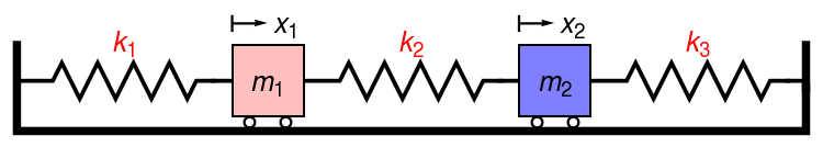
The model consists of two springs obeying Hooke's law and two weights. One
elastic spring, having spring constant k 1 , is attached to the ceiling and a weight of mass m 1 is attached to the lower end of this spring. To this weight, a second elastic spring is attached having spring constant k 2 . To the bottom of this second spring, a weight of mass m 2 is attached, and the entire system as illustrated in the figure at left.
Then such system is modeled by the following system of ordinary differential equations
\[
\begin{cases}
m_1 \ddot{x}_1 = - k_1 x_1 - k_2 \left( x_1 - x_2 \right) , \\
m_2 \ddot{x}_2 = - k_2 \left( x_2 - x_1 \right) ,
\end{cases}
\]
which leads to the following second order vector equation
\[
\ddot{\bf x} + {\bf A} \,{\bf x} = {\bf 0} , \qquad\mbox{where} \qquad
{\bf A} = \begin{bmatrix} \frac{k_1 + k_2}{m_1} & - \frac{k_2}{m_1} \\
\frac{k_2}{m_2} & \frac{k_2}{m_2} \end{bmatrix} = \begin{bmatrix} \phantom{-}3&-1 \\
-2&\phantom{-}2 \end{bmatrix} .
\tag{1.1}
\]
Suppose that the initial displacements and initial velocity are given
\[
x_1 (0) = x_{10}, \quad x_2 (0) = x_{20}, \qquad \dot{x}_1 (0) = v_{10},
\quad \dot{x}_2 (0) = v_{20} .
\tag{1.2}
\]
Then the solution of the given second order system of equations is
\[
\begin{bmatrix} x_1 (t) \\ x_2 (t) \end{bmatrix} = \cos \left(
\sqrt{\bf A}\,t \right) \begin{bmatrix} x_{10} \\ x_{20} \end{bmatrix}
+ \frac{\sin \left( \sqrt{\bf A}\,t \right)}{\sqrt{\bf A}}
\begin{bmatrix} v_{10} \\ v_{20} \end{bmatrix} .
\tag{1.3}
\]
Therefore, we need to build two matrices
\begin{align*}
{\bf \Phi} (t) &= \frac{\sin \left( \sqrt{\bf A}\,t \right)}{\sqrt{\bf A}} ,
\\
{\bf \Psi} (t) &= \cos \left( \sqrt{\bf A}\,t \right) .
\end{align*}
Since matrix
A has two positive eigenvalues
A = {{3, -1}, {-2, 2}}
Eigenvalues[A]
{4, 1}
We use Sylvester's formula. Accordingly, we find first Sylvester's auxiliary
matrices:
\[
{\bf Z}_1 = \frac{{\bf A} - 4\,{\bf I}}{1-4} = \frac{1}{3} \begin{bmatrix}
1&1 \\ 2&2 \end{bmatrix} ,
\qquad
{\bf Z}_4 = \frac{{\bf A} - {\bf I}}{4-1} = \frac{1}{3} \begin{bmatrix}
\phantom{-}2&-1 \\ -2& \phantom{-}1 \end{bmatrix} .
\tag{1.4}
\]
Z1 = (A - 4*IdentityMatrix[2])/(-3)
{{1/3, 1/3}, {2/3, 2/3}}
Z4 = (A - IdentityMatrix[2])/(3)
{{2/3, -(1/3)}, {-(2/3), 1/3}}
Next, we check our calculations to show that auxiliary matrices are
projections on the eigenspaces, that is, the product
Z 1 ·
Z 1 =
Z 1 remains the same/
Z1.Z1 - Z1
{{0, 0}, {0, 0}}
Similarly,
Z 4 ·
Z 4 =
Z 4 .
Z4.Z4 - Z4
{{0, 0}, {0, 0}}
Z4.Z1
{{0, 0}, {0, 0}}
This allows us to bulid matrix functions explicitly:
\begin{align*}
{\bf \Phi} (t) &= \frac{\sin \left( \sqrt{\bf A}\,t \right)}{\sqrt{\bf A}} =
\sin t \,{\bf Z}_1 + \frac{\sin 2t}{2}\, {\bf Z}_4 = \frac{\sin t}{3}
\begin{bmatrix}
1&1 \\ 2& 2 \end{bmatrix} + \frac{\sin 2t}{6} \begin{bmatrix}
\phantom{-}2&-1 \\ -2& \phantom{-}1 \end{bmatrix} ,
\\
{\bf \Psi} (t) &= \cos \left( \sqrt{\bf A}\,t \right) = \cos t\,{\bf Z}_1 +
\cos 2t\, {\bf Z}_4 = \frac{\cos t}{3} \begin{bmatrix}
1&1 \\ 2& 2 \end{bmatrix} + \frac{\cos 2t}{3} \begin{bmatrix}
\phantom{-}2&-1 \\ -2& \phantom{-}1 \end{bmatrix} .
\end{align*}
Finally, we represent the solution of the given problem explicitly:
\[
\begin{bmatrix}
x_1 (t) \\
x_2 (t) \end{bmatrix} = {\bf \Psi} (t) \begin{bmatrix}
x_{10} \\
x_{20} \end{bmatrix} + {\bf \Phi} (t) \begin{bmatrix}
v_{10} \\
v_{20} \end{bmatrix} .
\tag{1.4}
\]
Now we solve the same problem by transfering it into the system of first order
differential equations. Upon introducing new dependent variables
\[
y_1 = x_1 , \quad y_2 = x_2 , \quad y_3 = \dot{x}_1 = \dot{y}_1 , \quad
y_4 = \dot{x}_2 = \dot{y}_2 .
\]
Then for these new variables, we obtain the following system of differential
equation sof first order:
\begin{align*}
\dot{y}_1 &= y_3 , \\
\dot{y}_2 &= y_4 , \\
\dot{y}_3 &= -3\,y_1 + y_2 , \\
\dot{y}_4 &= 2\,y_1 -2\, y_2 ,
\end{align*}
which we rewrite in vector form:
\[
\frac{\text d}{{\text d}t}\,{\bf y} = {\bf B}\, {\bf y} \qquad\mbox{or} \qquad
\frac{\text d}{{\text d}t} \begin{bmatrix} y_1 \\ y_2 \\ y_3 \\ y_4
\end{bmatrix} + \begin{bmatrix} \phantom{-}0&\phantom{-}0&1&0 \\ \phantom{-}0&\phantom{-}0&0&1 \\ -3&\phantom{-}1&0&0 \\ \phantom{-}2&-2&0&0
\end{bmatrix} \begin{bmatrix} y_1 \\ y_2 \\ y_3 \\ y_4
\end{bmatrix} .
\]
The eigenvalues of matrix
B are
\( \lambda =
\pm {\bf j} , \quad \lambda = \pm 2{\bf j} . \)
B = {{0, 0, 1, 0}, {0, 0, 0, 1}, {-3, 1, 0, 0}, {2, -2, 0, 0}}
{2 I, -2 I, I, -I}
Since matrix
B is diagonalizable (it has four distinct simple
eigenvalues), we again can use Sylvester's formula. Right now we need to find
only two Sylvester's auxiliary matrices because two others are complex
conjugate. So
\begin{align*}
{\bf Z}_{j} &= \frac{\left( {\bf B} + {\bf j}\,{\bf I} \right) \left(
{\bf B}^2 + 4\,{\bf I} \right)}{\left( 2\,{\bf j} \right)\left( -1+4 \right)} =
\frac{1}{6} \begin{bmatrix} 1&1&-{\bf j}&-{\bf j} \\
2&2&-2{\bf j}&-2{\bf j} \\ {\bf j}&{\bf j} &\phantom{-}1 &\phantom{-}1 \\ 2{\bf j}&2{\bf j}& \phantom{-}2&\phantom{-}2
\end{bmatrix} ,
\\
{\bf Z}_{2j} &= \frac{\left( {\bf B} + 2{\bf j}\,{\bf I} \right) \left(
{\bf B}^2 + {\bf I} \right)}{\left( 4\,{\bf j} \right)\left( 4-1 \right)}
= \frac{1}{12} \begin{bmatrix} \phantom{-}4&-2&-2{\bf j}&\phantom{-}{\bf j} \\
-4&\phantom{-}2& \phantom{-}2{\bf j}&-{\bf j} \\ \phantom{-}8{\bf j}&-4{\bf j}&\phantom{-}4&-2 \\
-8{\bf j}&\phantom{-}4{\bf j}&-4&\phantom{-}2 \end{bmatrix} ,
\end{align*}
where
I is the identity 4×4 matrix.
Zj = (B + I*IdentityMatrix[4]).(B.B + 4*IdentityMatrix[4])/(2*I)/3
{{1/6, 1/6, -(I/6), -(I/6)}, {1/3, 1/3, -(I/3), -(I/3)}, {I/6, I/6, 1/
6, 1/6}, {I/3, I/3, 1/3, 1/3}}
Z2j = (B + 2*I*IdentityMatrix[4]).(B.B + IdentityMatrix[4])/(4*I)/(-3)
{{1/3, -(1/6), -(I/6), I/12}, {-(1/3), 1/6, I/6, -(I/12)}, {(2 I)/
3, -(I/3), 1/3, -(1/6)}, {-((2 I)/3), I/3, -(1/3), 1/6}}
These auxiliary matrices are orthogonal:
Zj.Z2j
{{0, 0, 0, 0}, {0, 0, 0, 0}, {0, 0, 0, 0}, {0, 0, 0, 0}}
and are projections:
Zj.Zj - Zj
{{0, 0, 0, 0}, {0, 0, 0, 0}, {0, 0, 0, 0}, {0, 0, 0, 0}}
Z2j.Z2j - Z2j
{{0, 0, 0, 0}, {0, 0, 0, 0}, {0, 0, 0, 0}, {0, 0, 0, 0}}
Now we build the exponential matrix
\[
{\bf U} (t) = e^{{\bf B}\,t} = 2\,\Re \,e^{{\bf j}t}\, {\bf Z}_{j} +
2\,\Re \,e^{2{\bf j}t}\, {\bf Z}_{2j} ,
\]
where Re = ℜ is the real part and Im = ℑ is the imaginary part of a
complex number. We can slightly simply the above formula with the aid of Euler
identity:
\( e^{{\bf j}\theta} = \cos\theta +
{\bf j}\,\sin\theta : \)
\[
{\bf U} (t) = e^{{\bf B}\,t} = 2\,\cos t \,\Re \,{\bf Z}_{j} - 2\,\sin t \,
\Im\,{\bf Z}_{j} + 2\,\cos 2t \,\Re \,{\bf Z}_{2j} - 2\,\sin 2t \,
\Im\,{\bf Z}_{2j} .
\]
To find its explicit value, we use
Mathematica :
U[t_]= 2*Cos[t]*Re[Zj] - 2*Sin[t]*Im[Zj] + 2*Cos[2*t]*Re[Z2j] - 2*Sin[2*t]*Im[Z2j]
\[
{\bf U} (t) = e^{{\bf B}\,t} = \frac{\cos t}{3} \begin{bmatrix} 1&1&0&0 \\ 2&2&0&0 \\ 0&0&1&1 \\ 0&0&2&2 \end{bmatrix} + \frac{\sin t}{3} \begin{bmatrix} \phantom{-}0& \phantom{-}0&1&1 \\ \phantom{-}0& \phantom{-}0&2&2 \\ -1&-1&0&0 \\ -2&-2&0&0 \end{bmatrix} + \frac{\cos 2t}{3} \begin{bmatrix} \phantom{-}2 &-1& \phantom{-}0&\phantom{-}0 \\ -2&\phantom{-}1&\phantom{-}0&\phantom{-}0 \\ \phantom{-}0&\phantom{-}0&\phantom{-}2&-1 \\ \phantom{-}0&\phantom{-}0&-2&\phantom{-}1 \end{bmatrix} + \frac{\sin 2t}{3} \begin{bmatrix} \phantom{-}0&\phantom{-}0&\phantom{-}1&-\frac{1}{2} \\ \phantom{-}0&\phantom{-}0&-1&\phantom{-}\frac{1}{2} \\ -4& \phantom{-}2 & \phantom{-}0&\phantom{-}0 \\ \phantom{-}4&-2&\phantom{-}0&\phantom{-}0 \end{bmatrix} .
\]
We check our answer with standard
Mathematica command
Simplify[U[t] - MatrixExp[B*t]]
{{0, 0, 0, 0}, {0, 0, 0, 0}, {0, 0, 0, 0}, {0, 0, 0, 0}}
Since the answer is the zero matrix, our calculations are correct.
■
Example 2: Two vertical springs with resistance
Example 2:
\[
\begin{cases}
m_1 \ddot{x}_1 = - \delta_1 \dot{x}_1 - k_1 x_1 - k_2 \left( x_1 - x_2 \right) , \\
m_2 \ddot{x}_2 = - \delta_1 \dot{x}_2 - k_2 \left( x_2 - x_1 \right) ,
\end{cases}
\]
Let
\( \delta_1 = \delta_2 = 0.2 . \)
Applying the Laplace transform, we get
\[
\lambda^2 \begin{bmatrix} x_1^L \\ x_2^L \end{bmatrix} -
\begin{bmatrix} \dot{x}_1 (0) \\ \dot{x}_2 (0) \end{bmatrix} -
\lambda \begin{bmatrix} x_1 (0) \\ x_2 (0) \end{bmatrix} + \lambda
\begin{bmatrix} \delta_1 & 0 \\ 0 & \delta_2 \end{bmatrix} \begin{bmatrix} x_1^L \\ x_2^L \end{bmatrix} - \begin{bmatrix} \delta_1 & 0 \\ 0 & \delta_2 \end{bmatrix} \begin{bmatrix} x_1 (0) \\ x_2 (0) \end{bmatrix} + \begin{bmatrix} 3&-1 \\ -2&2 \end{bmatrix} \begin{bmatrix} x_1^L \\ x_2^L \end{bmatrix} = \begin{bmatrix} 0 \\ 0 \end{bmatrix}.
\]
Solving this algebraic equation with respect to unknown Laplace transforms,
we obtain
\[
\begin{bmatrix} x_1^L \\ x_2^L \end{bmatrix} = \left( \lambda^2 {\bf I} +
\lambda \,{\bf B} + {\bf A} \right)^{-1} \left\{ \dot{\bf x} (0) +
{\bf B} \,{\bf x} (0) + \lambda \,{\bf x} (0) \right\} ,
\]
where
\[
{\bf B} = \begin{bmatrix} \delta_1 & 0 \\ 0 & \delta_2 \end{bmatrix} =
\frac{1}{10} \begin{bmatrix} 2 & 0 \\ 0 & 2 \end{bmatrix} , \qquad
{\bf A} = \begin{bmatrix} \frac{k_1 + k_2}{m_1} & - \frac{k_2}{m_1} \\
\frac{k_2}{m_2} & \frac{k_2}{m_2} \end{bmatrix} = \begin{bmatrix} \phantom{-}3&-1 \\ -2&\phantom{-}2 \end{bmatrix} .
\]
Using
Mathematica , we find the inverse matrix
\[
{\bf R} = \left( \lambda^2 {\bf I} + \lambda \,{\bf B} + {\bf A} \right)^{-1}
= \begin{bmatrix} \lambda^2 + 0.2\,\lambda +3 & -1 \\ -2& \lambda^2 +
0.2\,\lambda + 2 \end{bmatrix}^{-1} = \frac{1}{100 + 25\,\lambda +
126\,\lambda^2 + 50\,\lambda^3 + 25\,\lambda^4} \begin{bmatrix}
500 + 5\,\lambda + 25\,\lambda^2 & 25 \\ 50 & 75 + 5\,\lambda + 25\, \lambda^2 \end{bmatrix} .
\]
A = {{3, -1}, {-2, 2}}
{{(2 + s/5 + s^2)/(4 + s + (126 s^2)/25 + (2 s^3)/5 + s^4), 1/(
4 + s + (126 s^2)/25 + (2 s^3)/5 + s^4)}, {2/(
4 + s + (126 s^2)/25 + (2 s^3)/5 + s^4), (3 + s/5 + s^2)/(
4 + s + (126 s^2)/25 + (2 s^3)/5 + s^4)}}
This allows us to explicitly express solutions in terms of their Laplace transforms:
\[
{\bf x}^L = \frac{1}{100 + 25\,\lambda +
126\,\lambda^2 + 50\,\lambda^3 + 25\,\lambda^4} \begin{bmatrix}
500 + 5\,\lambda + 25\,\lambda^2 & 25 \\ 50 & 75 + 5\,\lambda + 25\, \lambda^2 \end{bmatrix} \begin{bmatrix}
\dot{x}_1 (0) + \left( \lambda + \delta \right) x_1 (0) \\
\dot{x}_2 (0) + \left( \lambda + \delta \right) x_2 (0)
\end{bmatrix}
\]
Hence
\begin{align*}
x_1^L &= \frac{\left( 500 + 5\,\lambda + 25\,\lambda^2 \right) \left( \dot{x}_1 (0) + \left( \lambda + \delta \right) x_1 (0) \right) + 25 \left( \dot{x}_2 (0) + \left( \lambda + \delta \right) x_2 (0) \right)}{100 + 25\,\lambda +
126\,\lambda^2 + 50\,\lambda^3 + 25\,\lambda^4}
\\
&= \frac{500 \left( \dot{x}_1 (0) + \delta\,x_1 (0) \right) + 25 \left( \dot{x}_2 (0) + \delta\,x_2 (0) \right) + \lambda \left[ 2500 \left( \dot{x}_1 (0) + \delta\,x_1 (0) \right) + 500\,x_1 (0) + 25\,x_2 (0) \right] + \lambda^2 25 \left( \dot{x}_1 (0) + \delta\,x_1 (0) \right) + 5\,\lambda^2 x_1 (0) + 25 \lambda^3 x_1 (0)}{100 + 25\,\lambda +
126\,\lambda^2 + 50\,\lambda^3 + 25\,\lambda^4}
\end{align*}
and
\begin{align*}
x_2^L &= \frac{50 \left[ \dot{x}_1 (0) + \left( \lambda + \delta \right) x_1 (0) \right] + \left( 75 + 5\,\lambda + 25\, \lambda^2 \right) \left( \dot{x}_2 (0) + \left( \lambda + \delta \right) x_2 (0) \right)}{100 + 25\,\lambda +
126\,\lambda^2 + 50\,\lambda^3 + 25\,\lambda^4}
\\
&= \frac{50 \left[ \dot{x}_1 (0) + \delta\,x_1 (0) \right] + 75 \left[ \dot{x}_2 (0) + \delta\,x_2 (0) \right] + \lambda \left[ 50\,x_1 (0) + 5\dot{x}_2 (0) + 5\delta \,x_2 (0) + 75\,x_2 (0) \right] + 25\,\lambda^2 \left[ \dot{x}_2 (0) + \delta\,x_2 (0) \right] + 5\lambda^2 x_2 (0) + 25\,\lambda^3 x_2 (0)}{100 + 25\,\lambda +
126\,\lambda^2 + 50\,\lambda^3 + 25\,\lambda^4} .
\end{align*}
Therefore, we need to find four inverse Laplace transforms that we obtain again with the aid of Mathematica :
InverseLaplaceTransform[1/(100 + 25*s + 126*s^2 + 10* s^3 + 25*s^4), s, t]
(2 E^(-t/10) (133 Sqrt[11] Sin[(3 Sqrt[11] t)/10] -
11 Sqrt[399] Sin[(Sqrt[399] t)/10]))/65835
InverseLaplaceTransform[s/(100 + 25*s + 126*s^2 + 10* s^3 + 25*s^4), s, t]
(E^(-t/10) (4389 Cos[(3 Sqrt[11] t)/10] -
4389 Cos[(Sqrt[399] t)/10] - 133 Sqrt[11] Sin[(3 Sqrt[11] t)/10] +
11 Sqrt[399] Sin[(Sqrt[399] t)/10]))/329175
InverseLaplaceTransform[s^2 /(100 + 25*s + 126*s^2 + 10* s^3 + 25*s^4), s, t]
-(1/1645875)
E^(-t/10) (4389 Cos[(3 Sqrt[11] t)/10] -
4389 Cos[(Sqrt[399] t)/10] +
6517 Sqrt[11] Sin[(3 Sqrt[11] t)/10] -
2189 Sqrt[399] Sin[(Sqrt[399] t)/10])
InverseLaplaceTransform[s^3 /(100 + 25*s + 126*s^2 + 10* s^3 + 25*s^4), s, t]
--(1/8229375)
E^(-t/10) (105336 Cos[(3 Sqrt[11] t)/10] -
434511 Cos[(Sqrt[399] t)/10] -
9842 Sqrt[11] Sin[(3 Sqrt[11] t)/10] +
3289 Sqrt[399] Sin[(Sqrt[399] t)/10])
Correspondingly, we introduce four auxiliary functions:
\begin{align*}
g_0 (t) &= {\cal L}^{-1} \left( 100 + 25\,\lambda +
126\,\lambda^2 + 50\,\lambda^3 + 25\,\lambda^4 \right)^{-1} = e^{-t/10}
\\
g_1 (t) &= {\cal L}^{-1} \left[ \frac{\lambda}{100 + 25\,\lambda +
126\,\lambda^2 + 50\,\lambda^3 + 25\,\lambda^4} \right] = e^{-t/10}
\\
g_2 (t) &= {\cal L}^{-1} \left[ \frac{\lambda^2}{100 + 25\,\lambda +
126\,\lambda^2 + 50\,\lambda^3 + 25\,\lambda^4} \right] = e^{-t/10}
\frac{-1}{1645875} \left[ 4389 \,\cos \frac{3\sqrt{11}\,t}{10} - 4389\,
\cos \frac{\sqrt{399}\,t}{10} + 6517 \sqrt{11}\, \sin \frac{3\sqrt{11}\,t}{10}
- 2189\sqrt{399}\, \sin \frac{\sqrt{399}\,t}{10} \right] H(t) ,
\\
g_3 (t) &= {\cal L}^{-1} \left[ \frac{\lambda^3}{100 + 25\,\lambda +
126\,\lambda^2 + 50\,\lambda^3 + 25\,\lambda^4} \right] = e^{-t/10}
\frac{-1}{8229375} \left[ 105336\,\cos \frac{3\sqrt{11}\,t}{10} -
434511 \, \cos \frac{\sqrt{399}\,t}{10} - 9842\,\sqrt{11} \,\sin \frac{3\sqrt{11}\,t}{10} + 3289 \,\sqrt{399}\,\sin \frac{\sqrt{399}\,t}{10} \right] H(t) .
\end{align*}
Using these functions, we express tye solution:
\begin{align*}
x_1 (t) &= K_0 g_0 (t) + K_1 g_1 (t) + K_2 g_2 (t) + K_3 g_3 (t) ,
\\
x_2 (t) &= N_0 g_0 (t) + N_1 g_1 (t) + N_2 g_2 (t) + N_3 g_3 (t) ,
\end{align*}
where
\[
K_0 = 500 \left( \dot{x}_1 (0) + \delta\,x_1 (0) \right) + 25 \left( \dot{x}_2 (0) + \delta\,x_2 (0) \right) , \qquad K_1 = 2500 \left( \dot{x}_1 (0) + \delta\,x_1 (0) \right) + 500\,x_1 (0) + 25\,x_2 (0) ,
\]
\[
K_2 = 25 \left( \dot{x}_1 (0) + \delta\,x_1 (0) \right) + 5\, x_1 (0) , \qquad K_3 = 25\,x_1 (0) ,
\]
and
\[
N_0 = 50 \left[ \dot{x}_1 (0) + \delta\,x_1 (0) \right] + 75 \left[ \dot{x}_2 (0) + \delta\,x_2 (0) \right] , \qquad N_1 = \left[ 50\,x_1 (0) + 5\dot{x}_2 (0) + 5\delta \,x_2 (0) + 75\,x_2 (0) \right] ,
\]
\[
N_2 = 25 \left( \dot{x}_2 (0) + \delta\,x_2 (0) \right) + 5\, x_2 (0) , \qquad N_3 = 25\,x_2 (0) .
\]
■
Example 3: Two masses with three springs
Example 3:
Show[Graphics[{{Thickness[0.01],
Line[{{0, 1.2}, {0, 0}, {11, 0}, {11, 1.2}}]}, {Thickness[0.005],
Line[{{0,
0.7}, {.5, .7}, {.625, .95}, {.875, .45}, {1.125, .95}, \
{1.375, .45}, {1.625, .95}, {1.875, .45}, {2.125, .95}, {2.375, .45}, \
{2.5, .7}, {2.98, .7}}]},
Text[Style["\!\(\*SubscriptBox[\(k\), \(1\)]\)", Large, Red], {1.5,
1.25}], {EdgeForm[Thick], Pink, Opacity[0.5],
Rectangle[{3, .2}]}, {Thickness[0.003],
Circle[{3.25, .125}, .075]}, {Thickness[0.003],
Circle[{3.75, .125}, .075]}, {Thickness[0.003],
Line[{{3, 1.4}, {3, 1.6}}]}, {Thickness[0.003],
Arrowheads[Medium], Arrow[{{3, 1.5}, {3.5, 1.5}}]},
Text[Style["\!\(\*SubscriptBox[\(x\), \(1\)]\)", Large], {3.75,
1.5}], Text[
Style["\!\(\*SubscriptBox[\(m\), \(1\)]\)",
Large], {3.5, .7}], {Thickness[0.005],
Line[{{4.02,
0.7}, {4.5, .7}, {4.625, .95}, {4.875, .45}, {5.125, .95}, \
{5.375, .45}, {5.625, .95}, {5.875, .45}, {6.125, .95}, {6.375, .45}, \
{6.5, .7}, {6.98, .7}}]},
Text[Style["\!\(\*SubscriptBox[\(k\), \(2\)]\)", Large, Red], {5.5,
1.25}], {EdgeForm[Thick], Blue, Opacity[0.5],
Rectangle[{7, .2}]}, {Thickness[0.003],
Circle[{7.25, .125}, .075]}, {Thickness[0.003],
Circle[{7.75, .125}, .075]}, {Thickness[0.003],
Line[{{7, 1.4}, {7, 1.6}}]}, {Thickness[0.003],
Arrowheads[Medium], Arrow[{{7, 1.5}, {7.5, 1.5}}]},
Text[Style["\!\(\*SubscriptBox[\(x\), \(2\)]\)", Large], {7.75,
1.5}], Text[
Style["\!\(\*SubscriptBox[\(m\), \(2\)]\)",
Large], {7.5, .7}], {Thickness[0.005],
Line[{{8.02,
0.7}, {8.5, .7}, {8.625, .95}, {8.875, .45}, {9.125, .95}, \
{9.375, .45}, {9.625, .95}, {9.875, .45}, {10.125, .95}, {10.375, \
.45}, {10.5, .7}, {11, .7}}]},
Text[Style["\!\(\*SubscriptBox[\(k\), \(3\)]\)", Large, Red], {9.5,
1.25}]}], ImageSize -> 750]
\[
\begin{cases}
m_1 \, \dfrac{{\text d}^2 x_1}{{\text d}\,t^2} + \left( k_1 + k_2 \right) x_1 - k_2 \,x_2 &=0 , \\
m_2 \, \dfrac{{\text d}^2 x_2}{{\text d}\,t^2} + \left( k_2 + k_3 \right) x_2 - k_3 \,x_1 &=0 , \\
\end{cases} \qquad \begin{bmatrix} x_1 (0) \\ x_2 (0) \end{bmatrix} = \begin{bmatrix} d_1 \\ d_2 \end{bmatrix} , \qquad
\begin{bmatrix} \dot{x}_1 (0) \\ \dot{x}_2 (0) \end{bmatrix} = \begin{bmatrix} v_1 \\ v_2 \end{bmatrix} ,
\]
where
\( x_1 (t) \) and
\( x_2 (t) \) are displacements of masses
\( m_1 \) and
\( m_1 ,\) respectively. Here
\( k_1 , \ k_2 , \ k_3 \) are spring constants, and
\( d_1 , \ d_2 \) are initial displacements,
\( v_1 , \ v_2 \) are initial velocities.
Applying the Laplace transform, we get
\begin{align*}
m_1 \left( \lambda^2 x_1^L - v_1 - \lambda\,d_1 \right) &= - \left( k_1 + k_2 \right) x_1^L + k_2 x_2^L ,
\\
m_2 \left( \lambda^3 x_2^L - v_2 - \lambda\,d_2 \right) &= - \left( k_1 + k_2 \right) x_2^L + k_3 x_1^L .
\end{align*}
We solve this system of algebraic equations with
Mathematica :
Solve[{m1*(lambda^2 *x1-v1-lambda*d1)+(k1+k2)*x1 == k2*x2, m2*(lambda^2 *x2 -v2-lambda*d2) +(k2+k3)*x2-k3*x1==0}, {x1, x2}]
{{x1 -> -((
m1 (k2 + k3 + lambda^2 m2) (d1 lambda + v1) +
k2 m2 (d2 lambda + v2))/(
k2 k3 - (k1 + k2 + lambda^2 m1) (k2 + k3 + lambda^2 m2))),
x2 -> (d1 k3 lambda m1 + d2 lambda (k1 + k2 + lambda^2 m1) m2 +
k3 m1 v1 + k1 m2 v2 + k2 m2 v2 + lambda^2 m1 m2 v2)/(k2^2 +
k2 lambda^2 (m1 + m2) + lambda^2 m1 (k3 + lambda^2 m2) +
k1 (k2 + k3 + lambda^2 m2))}}
This yields
\[
x_1^L = \frac{- \left( k_2 + k_3 + \lambda^2 m_2 \right) \left( -d_1 \lambda - m_1 v_1 \right) + k_2 \left( d_2 \lambda m_2 + m_2 v_2 \right)}{\left( k_1 + k_2 + \lambda^2 m_1 \right) \left( k_2 + k_3 + \lambda^2 m_2 \right) - k_2 k_3} ,
\]
\[
x_2^L = \frac{d_1 k_3 \lambda m_1 + d_2 k_1 \lambda m_2 + d_2 k_2 \lambda m_2 + d_2 \lambda^2 m_1 m_2 + k_3 m_1 v_1 + k_1 m_2 v_2 + k_2 m_2 v_2 + \lambda^2 m_1 m_2 v_2}{k_1 k_2 + k_2^2 + k_1 k_3 + k_2 \lambda^2 m_1 + k_3 \lambda^2 m_1 + \left( k_1 + k_2 \right) \lambda^2 m_2 + \lambda^4 m_1 m_2} .
\]
Then we apply the inverse Laplace transform to obtain the solution
InverseLaplaceTransform[-((
m1 (k2 + k3 + lambda^2 m2) (d1 lambda + v1) +
k2 m2 (d2 lambda + v2))/(
k2 k3 - (k1 + k2 + lambda^2 m1) (k2 + k3 + lambda^2 m2))), lambda,
t]
(E^(-((Sqrt[-(k1/m1) - k2/m1 - k2/m2 - k3/m2 -
Sqrt[-4 (k1 k2 + k2^2 + k1 k3) m1 m2 + (k2 m1 + k3 m1 + k1 m2 +
k2 m2)^2]/(m1 m2)] t)/Sqrt[2]) - (
Sqrt[-(k1/m1) - k2/m1 - k2/m2 - k3/m2 +
Sqrt[-4 (k1 k2 + k2^2 + k1 k3) m1 m2 + (k2 m1 + k3 m1 + k1 m2 +
k2 m2)^2]/(m1 m2)] t)/Sqrt[
2]) (Sqrt[2] d1 E^((
Sqrt[-(k1/m1) - k2/m1 - k2/m2 - k3/m2 -
Sqrt[-4 (k1 k2 + k2^2 + k1 k3) m1 m2 + (k2 m1 + k3 m1 + k1 m2 +
k2 m2)^2]/(m1 m2)] t)/Sqrt[2])
k2 m1 Sqrt[-(k1/m1) - k2/m1 - k2/m2 - k3/m2 -
Sqrt[-4 (k1 k2 + k2^2 + k1 k3) m1 m2 + (k2 m1 + k3 m1 + k1 m2 +
k2 m2)^2]/(m1 m2)]
Sqrt[-(k1/m1) - k2/m1 - k2/m2 - k3/m2 +
Sqrt[-4 (k1 k2 + k2^2 + k1 k3) m1 m2 + (k2 m1 + k3 m1 + k1 m2 +
k2 m2)^2]/(m1 m2)] -
Sqrt[2] d1 E^((
Sqrt[-(k1/m1) - k2/m1 - k2/m2 - k3/m2 +
Sqrt[-4 (k1 k2 + k2^2 + k1 k3) m1 m2 + (k2 m1 + k3 m1 + k1 m2 +
k2 m2)^2]/(m1 m2)] t)/Sqrt[2])
k2 m1 Sqrt[-(k1/m1) - k2/m1 - k2/m2 - k3/m2 -
Sqrt[-4 (k1 k2 + k2^2 + k1 k3) m1 m2 + (k2 m1 + k3 m1 + k1 m2 +
k2 m2)^2]/(m1 m2)]
Sqrt[-(k1/m1) - k2/m1 - k2/m2 - k3/m2 +
Sqrt[-4 (k1 k2 + k2^2 + k1 k3) m1 m2 + (k2 m1 + k3 m1 + k1 m2 +
k2 m2)^2]/(m1 m2)] -
Sqrt[2] d1 E^(
Sqrt[2] Sqrt[-(k1/m1) - k2/m1 - k2/m2 - k3/m2 -
Sqrt[-4 (k1 k2 + k2^2 + k1 k3) m1 m2 + (k2 m1 + k3 m1 +
k1 m2 + k2 m2)^2]/(m1 m2)] t + (
Sqrt[-(k1/m1) - k2/m1 - k2/m2 - k3/m2 +
Sqrt[-4 (k1 k2 + k2^2 + k1 k3) m1 m2 + (k2 m1 + k3 m1 +
k1 m2 + k2 m2)^2]/(m1 m2)] t)/Sqrt[2])
and
InverseLaplaceTransform[(d1 k3 lambda m1 +
d2 lambda (k1 + k2 + lambda^2 m1) m2 + k3 m1 v1 + k1 m2 v2 +
k2 m2 v2 + lambda^2 m1 m2 v2)/(k2^2 + k2 lambda^2 (m1 + m2) +
lambda^2 m1 (k3 + lambda^2 m2) +
k1 (k2 + k3 + lambda^2 m2)), lambda, t]
(E^(-((Sqrt[-(k1/m1) - k2/m1 - k2/m2 - k3/m2 -
Sqrt[-4 (k1 k2 + k2^2 + k1 k3) m1 m2 + (k2 m1 + k3 m1 + k1 m2 +
k2 m2)^2]/(m1 m2)] t)/Sqrt[2]) - (
Sqrt[-(k1/m1) - k2/m1 - k2/m2 - k3/m2 +
Sqrt[-4 (k1 k2 + k2^2 + k1 k3) m1 m2 + (k2 m1 + k3 m1 + k1 m2 +
k2 m2)^2]/(m1 m2)] t)/Sqrt[
2]) (-Sqrt[2] d2 E^((
Sqrt[-(k1/m1) - k2/m1 - k2/m2 - k3/m2 -
Sqrt[-4 (k1 k2 + k2^2 + k1 k3) m1 m2 + (k2 m1 + k3 m1 + k1 m2 +
k2 m2)^2]/(m1 m2)] t)/Sqrt[2])
k2 m1 Sqrt[-(k1/m1) - k2/m1 - k2/m2 - k3/m2 -
Sqrt[-4 (k1 k2 + k2^2 + k1 k3) m1 m2 + (k2 m1 + k3 m1 + k1 m2 +
k2 m2)^2]/(m1 m2)]
Sqrt[-(k1/m1) - k2/m1 - k2/m2 - k3/m2 +
Sqrt[-4 (k1 k2 + k2^2 + k1 k3) m1 m2 + (k2 m1 + k3 m1 + k1 m2 +
k2 m2)^2]/(m1 m2)] +
Sqrt[2] d2 E^((
Sqrt[-(k1/m1) - k2/m1 - k2/m2 - k3/m2 +
Sqrt[-4 (k1 k2 + k2^2 + k1 k3) m1 m2 + (k2 m1 + k3 m1 + k1 m2 +
k2 m2)^2]/(m1 m2)] t)/Sqrt[2])
k2 m1 Sqrt[-(k1/m1) - k2/m1 - k2/m2 - k3/m2 -
Sqrt[-4 (k1 k2 + k2^2 + k1 k3) m1 m2 + (k2 m1 + k3 m1 + k1 m2 +
k2 m2)^2]/(m1 m2)]
Sqrt[-(k1/m1) - k2/m1 - k2/m2 - k3/m2 +
Sqrt[-4 (k1 k2 + k2^2 + k1 k3) m1 m2 + (k2 m1 + k3 m1 + k1 m2 +
k2 m2)^2]/(m1 m2)] +
Sqrt[2] d2 E^(
Sqrt[2] Sqrt[-(k1/m1) - k2/m1 - k2/m2 - k3/m2 -
Sqrt[-4 (k1 k2 + k2^2 + k1 k3) m1 m2 + (k2 m1 + k3 m1 +
k1 m2 + k2 m2)^2]/(m1 m2)] t + (
Sqrt[-(k1/m1) - k2/m1 - k2/m2 - k3/m2 +
Sqrt[-4 (k1 k2 + k2^2 + k1 k3) m1 m2 + (k2 m1 + k3 m1 +
k1 m2 + k2 m2)^2]/(m1 m2)] t)/Sqrt[2])
We choose the following numewrical values:
\[
m_1 = 1\,\texttt{kg}, \quad m_2 = 2/3\,\texttt{kg}, \quad k_1 = 0.3\,\texttt{N/m}, \quad k_2 = 0.08\,\texttt{N/m}, \quad k_3 = 0.2\,\texttt{N/m},
\]
with the initial conditions
\[
d_1 = -0.08\,\texttt{m}, \quad d_2 = 0.4\,\texttt{m}, \quad v_1 = 0.15\,\texttt{m/sec}, \quad v_2 = -0.3\,\texttt{m/sec}.
\]
■
The Ideal Mass-Spring-Damper Systems
Force due to mechanical resistance or viscosity is typically approximated as being proportional to velocity:
F =
k v .
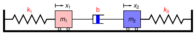
Example 4: Two masses with two springs and a dashpot subject to resistance
Example 4:
Show[dash, dash2, dash3,
Graphics[{{Thickness[0.01],
Line[{{0, 1.2}, {0, 0}, {11, 0}, {11, 1.2}}]}, {Thickness[0.005],
Line[{{0,
0.7}, {.5, .7}, {.625, .95}, {.875, .45}, {1.125, .95}, \
{1.375, .45}, {1.625, .95}, {1.875, .45}, {2.125, .95}, {2.375, .45}, \
{2.5, .7}, {2.98, .7}}]},
Text[Style["\!\(\*SubscriptBox[\(k\), \(1\)]\)", Large, Red], {1.5,
1.25}], {EdgeForm[Thick], Pink, Opacity[0.5],
Rectangle[{3, .2}]}, {Thickness[0.003],
Circle[{3.25, .125}, .075]}, {Thickness[0.003],
Circle[{3.75, .125}, .075]}, {Thickness[0.003],
Line[{{3, 1.4}, {3, 1.6}}]}, {Thickness[0.003],
Arrowheads[Medium], Arrow[{{3, 1.5}, {3.5, 1.5}}]},
Text[Style["\!\(\*SubscriptBox[\(x\), \(1\)]\)", Large], {3.75,
1.5}], Text[
Style["\!\(\*SubscriptBox[\(m\), \(1\)]\)", Large], {3.5, .7}],
Text[Style["b", Large, Red], {5.5, 1.25}], {EdgeForm[Thick], Blue,
Opacity[0.5], Rectangle[{7, .2}]}, {Thickness[0.003],
Circle[{7.25, .125}, .075]}, {Thickness[0.003],
Circle[{7.75, .125}, .075]}, {Thickness[0.003],
Line[{{7, 1.4}, {7, 1.6}}]}, {Thickness[0.003],
Arrowheads[Medium], Arrow[{{7, 1.5}, {7.5, 1.5}}]},
Text[Style["\!\(\*SubscriptBox[\(x\), \(2\)]\)", Large], {7.75,
1.5}], Text[
Style["\!\(\*SubscriptBox[\(m\), \(2\)]\)",
Large], {7.5, .7}], {Thickness[0.005],
Line[{{8.02,
0.7}, {8.5, .7}, {8.625, .95}, {8.875, .45}, {9.125, .95}, \
{9.375, .45}, {9.625, .95}, {9.875, .45}, {10.125, .95}, {10.375, \
.45}, {10.5, .7}, {11, .7}}]},
Text[Style["\!\(\*SubscriptBox[\(k\), \(3\)]\)", Large, Red], {9.5,
1.25}]}], ImageSize -> 750]
Suppose we have two point masses of mass m ₁, m ₂ and two hookean springs with spring constants k ₁, k ₃. Two masses are connected by dashpot as shown in the figure. The left end of spring 1 and the right end of spring 3 are attached to immovable surfaces. The masses are in contact with a surface whose coefficient of friction (damping constant) is δ (they could be different for each mass, but we assume that they are the same for simplicity). Their resitance is proportional to the velocities of point masses. We also assume that the mass of the springs is negligible, friction does not affect the springs. Hooke's law is applicable to the springs along only their horizontal motion. This leads to the following model:
\[
\begin{cases}
m_1 \, \dfrac{{\text d}^2 x_1}{{\text d}\,t^2} + \delta\,\dot{x}_1 + k_1 x_1 + b \left( \dot{x}_1 - \dot{x}_2 \right) &=0 , \\
m_2 \, \dfrac{{\text d}^2 x_2}{{\text d}\,t^2} + \delta\,\dot{x}_2 + b \left( \dot{x}_2 - \dot{x}_1 \right) + k_3 \,x_2 &=0 , \\
\end{cases} \qquad \begin{bmatrix} x_1 (0) \\ x_2 (0) \end{bmatrix} = \begin{bmatrix} d_1 \\ d_2 \end{bmatrix} , \qquad
\begin{bmatrix} \dot{x}_1 (0) \\ \dot{x}_2 (0) \end{bmatrix} = \begin{bmatrix} v_1 \\ v_2 \end{bmatrix} ,
\]
where
\( x_1 (t) \) and
\( x_2 (t) \) are displacements of masses
\( m_1 \) and
\( m_1 ,\) respectively. Here
\( k_1 , \ k_2 , \ k_3 \) are spring constants, and
\( d_1 , \ d_2 \) are initial displacements,
\( v_1 , \ v_2 \) are initial velocities.
We rewrite this system of ODEs in a vector form:
\[
\frac{{\text d}^2 {\bf x}}{{\text d} t^2} + {\bf B}\, \frac{{\text d} {\bf x}}{{\text d} t} + {\bf A}\,{\bf x} = {\bf 0}, \qquad {\bf x}(0) = {\bf d}, \quad \dot{\bf x}(0) = {\bf v} ,
\]
where
\[
{\bf A} = \begin{bmatrix} \frac{k_1}{m_1} & 0 \\ 0 & \frac{k_3}{m_2} \end{bmatrix} , \qquad {\bf B} = \begin{bmatrix} \frac{\delta + b}{m_1} & -\frac{b}{m_1} \\ -\frac{b}{m_2} & \frac{\delta + b}{m_2} \end{bmatrix} , \qquad {\bf x}(t) = \begin{bmatrix} x_1 (t) \\ x_2 (t) \end{bmatrix}
\]
We choose the following numewrical values:
\[
m_1 = 1\,\texttt{kg}, \quad m_2 = 2\,\texttt{kg}, \quad k_1 = 1\,\texttt{N/m}, \quad k_2 = 2\,\texttt{N/m}, \quad b = 0.5\,\texttt{Ns/m},
\]
with the initial conditions
\[
d_1 = 0.1\,\texttt{m}, \quad d_2 = 0.3\,\texttt{m}, \quad v_1 = 0.2\,\texttt{m/sec}, \quad v_2 = -0.5\,\texttt{m/sec}.
\]
■
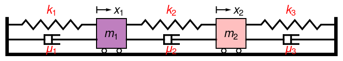
Example 5: Two masses with three springs and three dashpots subject to resistance
Example 5:
We need to take into accound resistive forces acting on each mass.
For example, the forces acting on mass 1 are −k 1 x 1 from spring 1 and k 2 (x 2 − x 1 ) from spring 2. When you add up all the forces, combine terms and set them equal to zero, you get the first equation in the system. A similar analysis is applied to the second mass to get the second equation.
\[
\begin{cases}
m_1 \frac{{\text d}^2 x_1}{{\text d}t^2} + \left( k_1 + k_2 \right) x_1 -k_2 x_2 &=0,
\\
m_2 \frac{{\text d}^2 x_2}{{\text d}t^2} + \left( k_2 + k_3 \right) x_1 -k_2 x_1 &=0
\end{cases}
\]
The frictional forces from the springs will be proportional to the velocity, so we have add velocity terms to incorporate the dashpot coefficients. These velocity terms are similar in arrangement to the
k x terms in the original equations since they also come from the springs. For example, if you imagine a diagram of the forces acting on the first mass, along with the spring forces from the previous equation, there will be a friction force from dashpot 1 of
\( -\mu_1 \dot{x}_1 , \)
as well as a friction force from dashpot 2 of
\( \mu_2 \left( \dot{x}_2 - \dot{x}_1 \right) . \)
The terms can be added and rearranged in terms of derivatives and the same
procedure applied to the second mass. The only forces acting on each mass are from the springsand the dashpots. After adding these dashpot friction forces to the systems of equationswe saw in class, the new system of equations is
\[
\begin{cases}
m_1 \frac{{\text d}^2 x_1}{{\text d}t^2} + \left( \mu_1 + \mu_2 \right) \frac{{\text d} x_1}{{\text d}t} - \mu_2 \frac{{\text d} x_2}{{\text d}t} + \left( k_1 + k_2 \right) x_1 -k_2 x_2 &=0,
\\
m_2 \frac{{\text d}^2 x_2}{{\text d}t^2} + \left( \mu_2 + \mu_3 \right) \frac{{\text d} x_2}{{\text d}t} - \mu_2 \frac{{\text d} x_1}{{\text d}t} + \left( k_2 + k_3 \right) x_1 -k_2 x_1 &=0
\end{cases}
\]
Show[Graphics[{{Thickness[0.01],
Line[{{0, 1.2}, {0, 0}, {11, 0}, {11, 1.2}}]}, {Thickness[0.005],
Line[{{0, 1}, {.5, 1}, {.625, 1.15}, {.875, .85}, {1.125,
1.15}, {1.375, .85}, {1.625, 1.15}, {1.875, .85}, {2.125,
1.15}, {2.375, .85}, {2.5, 1}, {2.98, 1}}]}, {Thickness[0.005],
Line[{{0, .5}, {1.25, .5}}]}, {Thickness[0.005],
Line[{{1.5, .5}, {3, .5}}]}, {Thickness[0.005],
Line[{{1.25, .35}, {1.25, .65}}]}, {Thickness[0.005],
Line[{{1.5, .35}, {1.5, .65}}]}, {Thickness[0.005],
Line[{{1.25, .35}, {1.75, .35}}]}, {Thickness[0.005],
Line[{{1.25, .65}, {1.75, .65}}]},
Text[Style["\*SubscriptBox[k, 1]", Large, Red], {1.5, 1.5}],
Text[Style["\*SubscriptBox[\[Mu], 1]", Large,
Red], {1.5, .2}], {EdgeForm[Thick], Purple, Opacity[0.5],
Rectangle[{3, .2}]}, {Thickness[0.003],
Circle[{3.25, .125}, .075]}, {Thickness[0.003],
Circle[{3.75, .125}, .075]}, {Thickness[0.003],
Line[{{3, 1.4}, {3, 1.6}}]}, {Thickness[0.003],
Arrowheads[Medium], Arrow[{{3, 1.5}, {3.5, 1.5}}]},
Text[Style["\*SubscriptBox[x, 1]", Large], {3.75, 1.5}],
Text[Style["\*SubscriptBox[m, 1]", Large], {3.5, .7}], {Thickness[
0.005], Line[{{4.02, 1}, {4.5, 1}, {4.625,
1.15}, {4.875, .85}, {5.125, 1.15}, {5.375, .85}, {5.625,
1.15}, {5.875, .85}, {6.125, 1.15}, {6.375, .85}, {6.5,
1}, {6.98, 1}}]}, {Thickness[0.005],
Line[{{4, .5}, {5.25, .5}}]}, {Thickness[0.005],
Line[{{5.5, .5}, {7, .5}}]},
{Thickness[0.005],
Line[{{5.25, .35}, {5.25, .65}}]}, {Thickness[0.005],
Line[{{5.5, .35}, {5.5, .65}}]}, {Thickness[0.005],
Line[{{5.25, .35}, {5.75, .35}}]}, {Thickness[0.005],
Line[{{5.25, .65}, {5.75, .65}}]},
Text[Style["\*SubscriptBox[k, 2]", Large, Red], {5.5, 1.5}],
Text[Style["\*SubscriptBox[\[Mu], 2]", Large,
Red], {5.5, .2}], {EdgeForm[Thick], Pink, Opacity[0.5],
Rectangle[{7, .2}]}, {Thickness[0.003],
Circle[{7.25, .125}, .075]}, {Thickness[0.003],
Circle[{7.75, .125}, .075]}, {Thickness[0.003],
Line[{{7, 1.4}, {7, 1.6}}]}, {Thickness[0.003],
Arrowheads[Medium], Arrow[{{7, 1.5}, {7.5, 1.5}}]},
Text[Style["\*SubscriptBox[x, 2]", Large], {7.75, 1.5}],
Text[Style["\*SubscriptBox[m, 2]", Large], {7.5, .7}], {Thickness[
0.005], Line[{{8.02, 1}, {8.5, 1}, {8.625,
1.15}, {8.875, .85}, {9.125, 1.15}, {9.375, .85}, {9.625,
1.15}, {9.875, .85}, {10.125, 1.15}, {10.37, .85}, {10.5,
1}, {11, 1}}]}, {Thickness[0.005],
Line[{{8, .5}, {9.25, .5}}]}, {Thickness[0.005],
Line[{{9.5, .5}, {11, .5}}]}, {Thickness[0.005],
Line[{{9.25, .35}, {9.25, .65}}]}, {Thickness[0.005],
Line[{{9.5, .35}, {9.5, .65}}]}, {Thickness[0.005],
Line[{{9.25, .35}, {9.75, .35}}]}, {Thickness[0.005],
Line[{{9.25, .65}, {9.75, .65}}]},
Text[Style["\*SubscriptBox[k, 3]", Large, Red], {9.5, 1.5}],
Text[Style["\*SubscriptBox[\[Mu], 3]", Large, Red], {9.5, .2}]}],
ImageSize -> 700]
The next step in the analysis is using software to find numerical solutions to these equations. It is convenient to use DSolve in Mathematica to solve the equations.
ClearAll;
(*units of N, N/m, m, kg, m/s*)
\[Mu]1 = 0.5;
\[Mu]2 = 1.4;
\[Mu]3 = 0.9;
k1 = 400;
k2 = 379;
k3 = 100;
m1 = 1;
m2 = 0.8;
d1 = 0.05;
d2 = 0.07;
v1 = 3;
v2 = 2;
eqn1 = m1*x''[t] + (\[Mu]1 + \[Mu]2)*x'[t] + \[Mu]2*y'[t] + (k1 + k2)*
x[t] - k2*y[t] == 0;
eqn2 = m2*y''[t] - \[Mu]1*x'[t] + (\[Mu]2 + \[Mu]3)*y'[t] -
k2*x[t] + (k2 + k3)*y[t] == 0;
eqns = {eqn1, eqn2, x[0] == d1, y[0] == d2, x'[0] == v1,
y'[0] == v2};
sol = DSolve[eqns, {x[t], y[t]}, t];
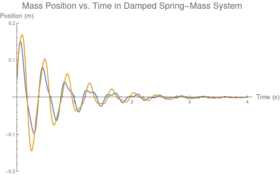
The next step is plotting the solutions to the equations with realistic values for the dashpots, springs, masses, initial displacements, and velocities. For Hookean springs, the spring constant can be calculated with the equation
F=k x . For example, if 5 N of force was applied to a spring and it displaced 2 cm, the spring constant would be
k = 250 N/m. The first test was to model a system with no friction, expecting to see an undamped oscillation. I used spring constants
k 1 = 200 N/m,
k 2 = 150 N/m, and
k 3 = 300 N/m. Iused masses of 1 kg and 0.5 kg, initial displacements of 5 cm and 3 cm, and initial velocitiesof 2 m/s and 1 m/s.
Here is Mathematica code:
Plot[{x[t] /. sol, y[t] /. sol}, {t, 0, 4}, PlotStyle -> Thick,
PlotRange -> {-.2, .2},
PlotLabel ->
Style["Mass Position vs. Time in Damped Spring-Mass System", 18],
PlotLegends -> {"Mass 1", "Mass 2"}, ImageSize -> Large,
AxesLabel -> {Style["Time (s)", 13], Style[ "Position (m)", 13]}]
Spring-mass oscillations.
Mathematica code
■
Driven spring-mass systems
Analysis of different spring-mass systems under sinusoidal excitation plays a
predominant role.
References
Return to Mathematica page main page (APMA0340) Part 1 Matrix Algebra Part 2 Linear Systems of Ordinary Differential Equations Part 3 Non-linear Systems of Ordinary Differential Equations Part 4 Numerical Methods Part 5 Fourier Series Part 6 Partial Differential Equations Part 7 Special Functions