Return to computing page for the second course APMA0340
Return to Mathematica tutorial for the first course APMA0330
Return to Mathematica tutorial for the second course APMA0340
Return to the main page for the first course APMA0330
Return to the main page for the second course APMA0340
Return to Part I of the course APMA0340
Introduction to Linear Algebra with Mathematica
Glossary
Inverted Pendulum
An inverted pendulum is not stable. Nevertheless, as pointed out by Pyotr Kapitza (1894--1984) in 1951, if you oscillate vertically the suspension point at a sufficientlyfast frequency Ω, you can stabilise it. A similar phenomenon occurs in a rotating saddle (see video), and is also used to create radio-frequency traps.
Let us start considering a very familiar one-dimensional system: a planar pendulum made of a massless rod of length ℓ ending with a point mass m. In the familiar swing, the driving occurs in different ways: if you “drive” the swing yourself, you do it by effectively modifying the position of your “center-of-mass”, hence the effective length ℓ(t) of the “pendulum”. If you are pushed by someone else, then you have a pendulum with a “periodic external force”. We use the generalize coordinate q = θ that denotes the angle formed with the vertical (θ = 0 being the downward position), and y0(t) denotes the position of its suspension point, we can derive the equations of motion from the Lagrangian formalism. In a short while we will assume that y0(t) = Acos Ωt, where A is the amplitude of the driving and Ω the driving frequency, but for the time being, let us proceed by keeping y0(t to be general. In a system of reference with the y-axis oriented upwards and the x-axis horizontally, the position x(t) and y(t) of the mass m is:
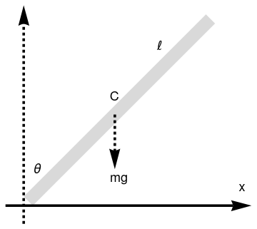
Example 1: If a rod or a pencil is held upright on a table, and then released, it will fall onto the ground. We consider a simple case when a rigid rod of length 2ℓ is fixed to a horizontal table by a smooth hinge at one end while another end is free to fall.
|
Falling pencil
rod = Graphics[{LightGray,
Polygon[{{0.1, 0}, {0, 0.1}, {2.0, 2.1}, {2.1, 2.0}}]}];
ar = Graphics[{Black, Thickness[0.01], Arrowheads[0.08], Arrow[{{-0.2, 0}, {2.5, 0}}]}]; ar2 = Graphics[{Black, Dashed, Thickness[0.01], Arrowheads[0.08], Arrow[{{0, -0.2}, {0, 2.2}}]}]; ar3 = Graphics[{Black, Dashed, Thickness[0.01], Arrowheads[0.08], Arrow[{{1, 1}, {1, 0.4}}]}]; tl = Graphics[{Black, Text[Style["\[ScriptL]", 18, FontFamily -> "Mathematica1"], {1.5, 1.75}]}]; tx = Graphics[{Black, Text[Style["x", 18], {2.4, 0.2}]}]; t1 = Graphics[{Black, Text[Style["C", 18], {1.0, 1.2}]}]; t2 = Graphics[{Black, Text[Style["\[Theta]", 18], {0.15, 0.4}]}]; t3 = Graphics[{Black, Text[Style["mg", 18], {1.05, 0.3}]}]; Show[rod, ar, ar2, ar3, tx, tl, t1, t2, t3] |
|
| Falling pencil. | Mathematica code |
Since the bottom end is hinged, there is no horizontal move of it. The kinetic energy, K, consists of the kinetic energy of the motion of the center of mass plus the kinetic energy of rotation about the bottom end of the pencil:
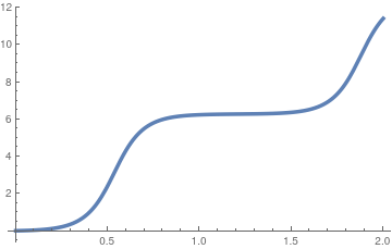
Let us consider a particular example of inverted pendulum that initially was displaced by 1° ·
Plot[Evaluate[y[t] /. sol], {t, 0, 2}, PlotStyle -> Thickness[0.01]]
|
|
|
||
| Initial velocity is 0.2; | Initial velocity is 1.2; | Initial velocity is 9,2. |
|
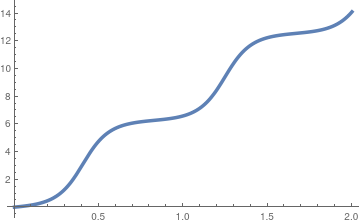
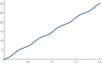
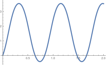
For a curious reader, we present the graph of the following initial value problem (IVP):
\[
\ddot{\theta} = 100\,\cos (\theta ) , \qquad \theta (0) = 0.0174533, \quad \dot{\theta} (0) = 0.2.
\]
sol2 = NDSolve[{y''[t] == 100*Cos[y[t]], y[0] == Pi/180,
y'[0] == 9.2}, y, {t, 0, 20}];
Plot[Evaluate[y[t] /. sol2], {t, 0, 2}, PlotStyle -> Thickness[0.01]] |
|
| Solution of the initial value problem d²θ/dt² = 100 cos(θ). | Mathematica code |
■
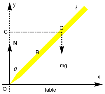
Example 2: Let us consider a stick or pencil or any elongated object of length ℓ is at at rest in upright position standing on frictionless table. Suppose that initial at time t = 0 it was pushed in the horizontal direction either by slight move or initial velocity or both. This will cause the pencil to fall, with bottom end sliding along the ground surface. Since there is no horizontal force acting on the object, its center of mass G moves only vertically. One generalized coordinate is enough to determine the state of the system. Let it be θ, the angle between the vertical axis and the pencil.
|
Falling pencil on ficktionless table:
pencil = Graphics[{Yellow,
Polygon[{{0.3, 0.2}, {0, 0}, {0.2, 0.3}, {2.0, 2.1}, {2.1,
2.0}}]}];
ar = Graphics[{Black, Thickness[0.01], Arrowheads[0.08],
Arrow[{{-0.2, 0}, {2.5, 0}}]}];
ar2 = Graphics[{Black, Dashed, Thickness[0.01], Arrowheads[0.08],
Arrow[{{0, -0.2}, {0, 2.2}}]}];
ar3 = Graphics[{Black, Dashed, Thickness[0.01], Arrowheads[0.08],
Arrow[{{1.4, 1.4}, {1.4, 0.8}}]}];
ar4 = Graphics[{Black, Thickness[0.01], Arrowheads[0.08],
Arrow[{{0, 0}, {0, 1.1}}]}];
tl = Graphics[{Black,
Text[Style["\[ScriptL]", 18, FontFamily -> "Mathematica1"], {1.8,
2.05}]}];
tx = Graphics[{Black, Text[Style["x", 18], {2.4, 0.2}]}];
t1 = Graphics[{Black, Text[Style["G", 18], {1.4, 1.5}]}];
t2 = Graphics[{Black, Text[Style["\[Theta]", 18], {0.15, 0.4}]}];
t3 = Graphics[{Black, Text[Style["mg", 18], {1.45, 0.5}]}];
t4 = Graphics[{Black, Text[Style["R", 18], {0.75, 0.85}]}];
t5 = Graphics[{Black, Text[Style["C", 18], {-0.1, 1.4}]}];
t6 = Graphics[{Black, Text[Style["N", Bold, 18], {0.15, 1.1}]}];
t7 = Graphics[{Black, Text[Style["O", 18], {-0.13, -0.13}]}];
t8 = Graphics[{Black, Text[Style["y", 18], {0.13, 2.13}]}];
t9 = Graphics[{Black, Text[Style["table", 18], {1.1, -0.15}]}];
line = Graphics[{Black, Dashed, Thick, Line[{{1.4, 1.4}, {0, 1.4}}]}];
Show[pencil, ar, ar2, ar3, ar4, tx, tl, t1, t2, t3, t4, t5, t6, t7,
t8, t9, line]
|
|
| Fig. 2.1: Falling pencil on fricktionless table. | Mathematica code |
To derive the equation of motion, we will denote by ω = dθ/dt the derivative of θ(t) with respect to time, and by α = dω/dt its acceleration. Let O denote a reference point of contact of the rod with the table, which moves in the horizontal direction. So its vector ro has only one coordinate in the x-direction; the vector rg describing the center of mass has only one coordinate in the y-direction. Let Ao denote the angular momentum of the system with respect to O as follows:
|
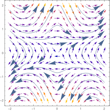
We plot the direction field for Eq.(5):
Table[VectorPlot[{y, (0.5*Sin[x] - 1/0.5*y^2*Cos[x]*Sin[x])/(1/3 +
Sin[x]^2)}, {x, -2, 2}, {y, -2, 2}, StreamPoints -> Coarse,
StreamScale -> {Full, All, 0.05}, StreamStyle -> "Arrow"]]
|
|
| Fig. 2.2: Direction field of the falling pencil on frickless table. | Mathematica code |
Now we rederive Eq.(2.5) using another point, C, as an instantaneous center of rotation. The corresponding moment of inertia is
|
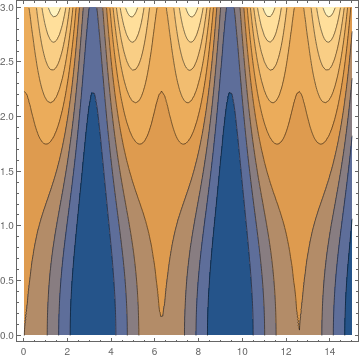
We plot the phase trajectories using Mathematica:
ContourPlot[(1 + 3*(Sin[x])^2)*y^2 /2 + 5*Cos[x], {x, 0, 15}, {y, 0,
3}, ContourStyle -> Black]
|
|
| Fig. 2.3: Phase portrait of the falling pencil on ficktionless table. | Mathematica code |
■
Example 3: ■
- Abalmassov, V.A., Maljutin, D.A., Where will a pen fall to?, School Teacher in Physics
- Bundy, F.P., Stresses in freely falling chimneys columns, Journal of Applied Physics, 1940, 11, No. 2, pp. 112--123.
- Crawford, F.S.,Moments to remember, American Journal of Physics, 1989, 57, Issue 2, p. 177. https://doi.org/10.1119/1.16117
- Cross, R., The fall and bounce of pencil and other elongated objects, American Journal of Physics, 2006, 74, Issue 1, pp. 26--30. https://doi.org/10.1119/1.2121752
- Cross, R., A falling rod on wheels, Physics Education, 2021, vol. 56, September, 5pp.
- Härtel, H., The falling stick with 𝑎 > g, The Physics Teacher, 2000, 38, January, pp. 54--55. https://doi.org/10.1119/1.880430
- Madson, E.L., Theory of the chimney breaking while falling, American Journal of Physics, 1977, 45, No. 2, pp. 182--184. https://doi.org/10.1119/1.10651
- Oliveira, V., Experiments with a falling rod, American Journal of Physics, 2016, 84, Issue 2, pp. 113--117. https://doi.org/10.1119/1.4934950
- Theron, W., The "faster than gravity" demonstration revisited, American Journal of Physics, 1988, 56, Issue 8, pp. 736--739. https://doi.org/10.1119/1.15513
- Tiersten, M.S., Moments not to forget---The conditions for equating torque and rate of change of angular momentum around the instantaneous center, American Journal of Physics, 1991, 59, pp. 733--738. https://doi.org/10.1119/1.16752
- Tiersten, M.S., Erratum: Moments not to forget---The conditions for equating torque and rate of change of angular momentum around the instantaneous center, American Journal of Physics, 1992, 60, No. 2, p. 187.
- Turner, L., Pratt, J.L., Does a falling pencil levitate?, Quantum, 1998, 8, No. 4, pp. 22-25. Online at National Science Teachers Association: https://www.nsta.org/quantum-magazine-math-and-science
- Varieschi, G, and Kamiya, K., Toy models for the falling chimney, American Journal of Physics, 2003, 71, No, 9, pp. 1025--1031. https://doi.org/10.1119/1.1576403
- Zypman, F.R., Moments to remember---The conditions for equating torgue and rate of change of angular momentum, American Journal of Physics, 1990, 58, No. 1, pp.41--43.
- Bukov, Martin, D’Alessio, Luca, and Polkovnikov, Anatoli, Universal high-frequency behavior of periodically driven systems: from dynamical stabilization to floquet engineering, Advances in Physics, 64(2):139–226, 2015.
- Kapitza, P. L., “Dynamic stability of the pendulum with vibrating suspension point, Sov. Phys. – JETP 21, 588–597 (1951) (in Russian). See also Collected papers of P. L. Kapitza, edited by D. Ter Haar ( Pergamon, London, 1965), Vol. 2, pp. 714–726.
- F. M. Phelps III and J. H. Hunter, Jr., An analytical solution of the inverted pendulum, American Journal of Physycs, 1965, 33, 285–295 (1965); https://doi.org/10.1119/1.1971474
- F. M. Phelps, III and J. H. Hunter, Jr., Am. J. Phys. 34, 533–535 (1966). https://doi.org/10.1119/1.1973087,
Return to Mathematica page
Return to the main page (APMA0340)
Return to the Part 1 Matrix Algebra
Return to the Part 2 Linear Systems of Ordinary Differential Equations
Return to the Part 3 Non-linear Systems of Ordinary Differential Equations
Return to the Part 4 Numerical Methods
Return to the Part 5 Fourier Series
Return to the Part 6 Partial Differential Equations
Return to the Part 7 Special Functions