Return to computing page for the first course APMA0330
Return to computing page for the second course APMA0340
Return to Mathematica tutorial for the first course APMA0330
Return to Mathematica tutorial for the second course APMA0340
Return to the main page for the first course APMA0330
Return to the main page for the second course APMA0340
Return to Part V of the course APMA0340
Introduction to Linear Algebra with Mathematica
Andrey Kolmogorov (1903--1987) from Moscow University (Russia), as a student at the age of 19, in his very first scientific work, constructed an example of an absolutely integrable function whose Fourier series diverges almost everywhere (later improved to diverge everywhere).
It turns out that many interesting problems in Fourier analysis do not depend
on the pointwise convergence. The Euler--Fourier formulas tacitly assume that the function is integrable in some sense. Therefore, we may consider Fourier series based on integration in Riemann, Lebesgue, Denjoy–Khinchin, and some other senses.
Actually, Fourier series is
based on another type of convergence, called 𝔏² convergence, where integration is assumed to be performed in Lebesgue sense. In order to make our presentation less technically demanding, we mostly use Riemann integration.
Of
course pointwise convergence is important for Fourier series; however, it is
more convenient to use Cesàro summation, which is a topic of the following section.
Fourier series of a periodic function f(x) can be considered as a transformation that assigns to function f(x) a sequence of its Fourier coefficients.
Since restoring a function from its Fourier series (or more precisely, from the set of its Fourier coefficients) is an ill-posed problem, we cannot expect that finite partial Fourier sums always converge to the generating this series function. As it was shown in the previous section, a pointwise convergence of Fourier series is a very delicate matter. Usually, ill-posed problems require some sort of regularization, and correspondingly Fourier series expansions were analyzed deeply and several regularizations are known.
In this section we discuss two basic types of convergence for series with functional coefficients---uniform convergence and convergence in mean (or 𝔏) sence. It was shown in 1873 by du Bois-Reymond that there exists a continuous function whose Fourier series diverges at some point. The 𝔏¹-case is even more pathological, as Kolmogorov was able to construct in 1923 an 𝔏¹-function whose Fourier series diverges pointwise almost everywhere.
In 1913, Nikolai Luzin conjectured that every function in 𝔏²([−ℓ, ℓ]) has an almost everywhere convergent Fourier series. Banach and Steinhauss proved in 1918 that there is no convergence in the 𝔏¹-norm. In 1966, Lennart Carleson managed to prove what was an authentic surprise for everybody: Luzin’s conjecture is true.
From that moment, the fact that the Fourier series of a function in 𝔏²([−ℓ, ℓ]) converges almost everywher was known as Carleson’s theorem. The next year, Richard Hunt extended the almost everywhere convergence to 𝔏p([−π,π]) for 1< p<∞.
The proof of Carleson was difficult to understand. Charles Fefferman, in 1973, proved Carleson’s theorem again. His methods were distinct to those of Carleson, but againdifficult to follow. Later, in the context of their work in multilinear harmonic analysis Lacey and Thiele came up with a quite short and easy to understand proof for the 𝔏² theorem that is to some extent a descendant of Fefferman's proof. They also wrote an expository article describing this and a number of related results.
Since we know that for existence of Fourier coefficients the function must be integrable over the interval of full period, the Fourier series should be considered for integrable functions.
The set of Riemann integrable functions is the most general class of functions we will be concerned with.
Such functions are bounded, but may have infinitely many discontinuities.
We recall that a real-valued function f
defined on some finite closed interval [𝑎, b] is Riemann integrable (which we abbreviate as integrable) if it is bounded, and if for every ε > 0, there is a subdivision [𝑎 = x0 < x1 < ··· < xN-1 < x1 = b of the interval [𝑎, b], so that if
\[
U = \sum_{j=1}^N \left[ \sup_{x_{j-1} \le x \le x_j} f(x) \right] \left( x_j - x_{j-1} \right) , \qquad
L = \sum_{j=1}^N \left[ \inf_{x_{j-1} \le x \le x_j} f(x) \right] \left( x_j - x_{j-1} \right) ,
\]
then we have U−L < ε.
We consider in convergent section three (another one will be considered separately in Cesàro section) kinds of convergence related to the Fourier series:
We say that the series \( \sum_{n\ge 0} f_n (x) \) converges to f(x) pointwise in the interval (𝑎, b), if for each \( x \in (a,b) \)
That is, the overall “distance” between the function f(x) and the partial sums \( F_N (x) = \sum_{n= 0}^N f_n (x) \) converges
to zero. Notice that the endpoints of the interval are included in the definition.
We say that the series \( \sum_{n\ge 0} f_n (x) \) converges to f(x) in the mean-square (or 𝔏² sense) in (𝑎, b), if
That is, the the “distance” between f(x) and the partial sums in the mean-square sense
converges to zero. ■
It is obvious from the definition that uniform convergence is the strongest of
the three, since uniformly convergent series will clearly converge pointwise,
as well as in the 𝔏² sense. The converse is not true, since
not every pointwise or 𝔏² convergent series is uniformly
convergent. Between the pointwise and 𝔏² convergence, neither is
stronger than the other, since there are series
that converge pointwise, but not in 𝔏², and vice versa.
The Euler--Fourier formulas \eqref{EqFourier.2} or \eqref{EqFourier.4} show that the Fourier coefficients are evaluated
as integrals over the whole interval where a function is defined (it is
convenient to integrate over symmetrical interval [−ℓ ,ℓ] because the function is extended periodically). Therefore,
these coefficients are influenced by the behavior of the function over the
interval. This is completely different from Taylor series where coefficients
are determined by the infinitesimal behavior of the function at the center of
expansion because they are calculated as derivatives at the point. On the
other hand, integral does not depend on the value of integrand function at
discrete number of points. So it is expected that we cannot restore the value
of the function at particular point from its Fourier series---Fourier
coefficients do not contain this information. In contrust, Taylor series
provide such information and pointwise or uniform convergence is appropriate
for them. Fourier series are based on another convergence that is called
𝔏² (square mean), and it is completely different type of
convergence. The advantage of this convergence is obvious: discontinuous functions could be expanded into Fourier series but not into Taylor series.
Theorem 2: Let f(x) be a square integrable function on the interval [−ℓ, ℓ], that is, \( \| f \|^2 = \int_{_\ell}^{\ell} |f(x)|^2 {\text d}x < \infty . \) Then the Fourier series for his function \( f(x) \,\sim \, \frac{a_0}{2} + \sum_{k\ge 0} \left[ a_k \cos \frac{k \pi x}{\ell} + b_k \sin \frac{k \pi x}{\ell} \right] , \)
where its coefficients are determined via Euler--Fourier formulas \eqref{EqFourier.4},
converges to f(x) in the mean square sense. ⧫
If we were to assume that the Fourier series of functions f converge to f in an appropriate sense, then we could infer that a function is uniquely determined by its Fourier coefficients. This would lead to the following statement: if f and g have the same Fourier coefficients, then f and g are necessarily equal. By taking the difference f − g, this proposition
can be reformulated for the zero function. As stated,
this assertion cannot be correct without reservation, since calculating
Fourier coefficients requires integration, and, for example,
any two functions which differ at finitely many points have the same
Fourier series.
Theorem 4:
Let f(x) be an integrable function (in the Lebesgue sense) on a symmetrical interval [−ℓ, ℓ]. If all its Fourier coefficients are zeroes, then f(x) = 0 whenever f is continuous at the
point x.
A Swedish mathematician Lennart Axel Edvard Carleson (born 1928) who showed in 1966, among
other things, that
if f is integrable in either the Riemann or Lebesgue sense, then the Fourier series
of f converges to f except possibly on a set of “measure 0.”
Corollary:
Let f(x) be continuous and periodic on the interval [−ℓ, ℓ], f(−ℓ) = f(ℓ), and suppose that the Fourier series of f(x) converges uniformly there. Then it converges to f(x).
Corollary:
If f(x) is continuous on the interval [−ℓ, ℓ], f(−ℓ) = f(ℓ), and all its Fourier coefficients are zeroes, then f(x) ≡ 0.
Let { 𝑎n }n≥0 be a sequence of (real or) complex numbers. We say that \( \sum_{n\ge 0} a_n \) converges to L if
\[
\lim_{N\to\infty} \sum_{n=0}^N a_n = L .
\]
We say that \( \sum_{n\ge 0} a_n \) converges absolutely if \( \sum_{n\ge 0} \vert a_n \vert \) converges. In case \( \sum_{n\ge 0} a_n \) converges, but does not converge absolutely, we say that \( \sum_{n\ge 0} a_n \) converges conditionally or is conditionally convergent. Note that absolute convergence implies convergence,
but that the converse fails.
The expression \( A_N = \sum_{n= 0}^N a_n \) is called the N-th partial sum (however, it is more common apply this definition to sums that start from 1, as \( A_N = \sum_{n= 1}^N a_n \) ).
Lemma 1: (Summation by parts)
For 1 ≤ j ≤ N, consider complex or real numbers
𝑎j and bj, with \( B_N = \sum_{n= 1}^N b_n . \) Then
Corollary 1:
Suppose 𝑎n → 0 and that
\( \sum_{n\ge 0} \left\vert a_{n+1} - a_n \right\vert \) converges. Assume also that the sequence { BN } of partial sums is bounded. Then \( \sum_{n\ge 0} a_{n} b_n \) converges.
Corollary 2:
Suppose 𝑎n decreases monotonically to 0. Then
\( \sum_{n\ge 0} (-1)^n a_n \) converges.
Suppose { fn } is a sequence of continuous functions on
[0, 1] (it can be any finite interval not necessarily [0, 1]). We assume that \( \lim_{n \to \infty} f_n (x) = f(x) \) exists for every x∈[0, 1], and inquire as to the nature of the limiting function f(x).
If we suppose that the convergence is uniform, matters are straight-forward and
f is then everywhere continuous. However, once we drop the assumption of uniform convergence, things may change radically and the issues that arise can be quite subtle. An example of this is given by the fact that one can construct a sequence of continuous functions { fn(x) }
converging everywhere to f(x) so that it is not Riemann integrable. So the relation
Here T = 2ℓ is the period and «P.V.» abbreviates the Cauchy principle value. As usual, j denotes the imaginary unit vector on complex plane ℂ, so j² = −1. These coefficients are related via the Euler formula:
Of course, two series in Eq.\eqref{EqMode.1} are equal under certain conditions. For example, they are equal
when both series converge uniformly.
Since expansion \eqref{EqMode.1} is a series representation of a function f(x) with respect to eigenfunctions of the Sturm--Liouville problem with periodic boundary conditions, this function f(x) should match these boundary conditions. In other words, Fourier series expansion \eqref{EqMode.1} is valid only for functions that are periodicly expanded for all x.
Therefore, Fourier series representations \eqref{EqMode.1} can be considered as
the inverse transformation 𝔉−1 of the assignment to a function a sequence of Fouriser coefficients according to Eqs.\eqref{EqMode.2} or (3):
The set of all functions having finite mean square norm is usually denoted by 𝔏²([−ℓ, ℓ]) (notations L² and L2 are also in use).
The most important in practice is the pointwise convergence of Fourier series, which was
discussed in the previous section. Uniform convergence easily implies pointwise convergence, 𝔏²-convergence and 𝔏¹-convergence. However, pointwise convergence is weakly related to the mean square convergence because discrete values of a function does not effect its integral value. Therefore, we analyze a relationship between pointwise convergence and convergence in mean.
In 1873, Paul du Bois-Reymond (1831--1889) showed that there exists a continuous function whose Fourier series diverges at a point. His example indicates that a continuous function cannot be recovered from its Fourier series expansion. However, this ill-posed problem later in 1900 was solved by Lipót Fejér (1880--1956) who used Cesàro summability method to confirm uniform convergence of Fourier partial sums for a continuous periodic function. He also proved that if a trigonometric series converges to an integrable function, it must be its Fourier series.
With Lebesguediscovery in 1902, his integration introduced new functional spaces, denoted by 𝔏p. The cases p = 1 and p = ∞ on p-mean convergence were proven negative, meaningthat there exists a function in 𝔏p such that its Fourier series does not converge in p-mean for these p, whereas the rest of cases were proven positive by Frigyes Riesz (1880--1956) in 1923, meaning that every function in 𝔏p has a Fourier series which is convergent in p-mean for 1 < p < ∞. His proof was based on the the theorem discovered in 1907 by him and Ernst Sigismund Fischer (1875--1954) that established the completeness of spaces 𝔏p.
In 1923, Andrew Kolmogorov (1903--1987) gave an example of integrable function, that is from 𝔏¹, such that its Fourier series diverges almost everywhere. Therefore, the case p=1 was dismissed. The case p=2 was conjecturedto be true by N.N. Luzin (1883--1950) in 1915 and proven true by Lennart Carleson (born 1928) in 1965. The result was later generalized by Richard Hunt (1937--2009), who in 1967 showed that there is convergence in 𝔏p for every p > 1.
Essentially, the biggest space in which the convergence of the Fourier series of anyfunction has been proven is, as done by Antonov in 1996. The smallest space in which it has been proven that there exists a function whose Fourier series diverges is, as proven by Konyagin in 2000.
Since a Fourier series for a function f(x) gives its periodic expansion, we can consider all function to be periodic with period 2ℓ.
For 1 ≤ p < ∞, define 𝔏p[−ℓ, ℓ] to be the set of all measurable functions f: [−ℓ, ℓ] → ℂ (or ℝ) such that
\[
\| f \|_p = \left( \int_{-\ell}^{\ell} \left\vert f(x) \right\vert^2 {\text d} x \right)^{1/p} < \infty ,
\]
This set becomes a Banach space when equipped with the norm above.
Technically, as a normed linear space, the 𝔏p space should consist of equivalence classes of such functions, where two functions are equivalent if and only if they differ on a set of measure zero. This is because a function that is zero only almost everywhere, under this definition, will still have norm zero. However, we can usually refer to an element of an 𝔏p space as a function instead of an equivalence class of functions without much trouble. Also, to be complete, integration in the definition of the norm should be understood in Lebesgue sense rather than in Riemann one.
Andrew Kolmogorov proved in 1923 that there exists an integrable function, that is from 𝔏¹, such that its Fourier series diverges almost everywhere. Therefore, the case p=1 was dismissed. The case p=2 was conjectured to be true by N. Luzin in 1915 and proven true by L. Carleson in 1965. The result was later generalized by Richard Hunt, who in 1967 showed that there is convergence in 𝔏p for every p > 1.
We know that convergence of Fourier series is justified in some function space (still unknown) that is situated between spaces 𝔏p ⊂ 𝔏¹. Nikolai Antonov discovered in 1996 a lower bound, and S.V. Konyagin introduced the space ℒφℒ as the upper bound. Therefore, we know that The Fourier convergence occurs for a function space bounded by these bounds: 𝔏p ⊂ A ⊂ ℒφℒ ⊂𝔏¹.
Theorem 2:
Suppose f is a periodic function of period 2ℓ that belong to the class 𝔏p[−ℓ, ℓ], with 1 < p < ∞ . Then its Fourier partial sums converge to f in 𝔏p sense:
\[
\lim_{n\to \infty} \left( \int_{-\ell}^{\ell} \left\vert S_n (f)(x) - f(x) \right\vert^p {\text d} x \right)^{1/p} = O .
\]
\[
\| f \| = \sqrt{\langle f, f \rangle} = \left( \int_{-\ell}^{\ell} \left\vert f(x) \right\vert^2 {\text d} x \right)^{1/2} .
\]
For a function in 𝔏²(−ℓ, ℓ) its trigonometric Fourier series converges almost everywhere. This was stated as a conjecture by N. Luzin in 1915 and proven true by L. Carleson in 1965.
We are going to prove this statement assuming that trigonometric polynomials are dense in 𝔏².
Theorem 3:
Let f be a square-integrable function, f ∈ 𝔏²([−ℓ, ℓ]). A trigonometric polynomial of degree N that best approximates f in the norm ||·||2 is the Nth Fourier sum \eqref{EqMode.4} of f.
The first two terms of the last expression do not depend on p(x), whereas the last one does. Since all the terms in the last term are positive, the only choice to minimize it is to set ck = 𝑎k and dk = bk for every k
Theorem 4 (Bessel inequality:
Let f ∈ 𝔏²([−ℓ, ℓ]). Then
Since this inequality holds for every N, it also does for the limit N → ∞.
Since infinite sums of squares of Fourier coefficients converge, we immediately deduce that Riemann-Lebesgue lemma is valid for functions from
𝔏²(−ℓ, ℓ):
Since we discuss expansions of functions into Fourier series, we need a special space of functions that is suitable for this task. Previously, we introduced the space of absolutely integrable functions 𝔏¹([−ℓ, ℓ]) with the norm
To handle Fourier series, we need a subspace of this space that is denoted as 𝔏²([−ℓ, ℓ]) ⊂ 𝔏¹([−ℓ, ℓ]). The norm in 𝔏² is generated by the inner product
The inner product of two functions f and g, denoted either by \( \langle f(x) , g(x) \rangle \) in mathematics or \( \langle f(x) \,|\, g(x) \rangle \) in physics and engineering, is defined as
\[
\langle f(x) \,|\, g(x) \rangle = \int_{-\ell}^{\ell} \overline{f(x)}g(x)\,{\text d} x = \int_{-\ell}^{\ell} f(x)^{\ast} g(x)\,{\text d} x ,
\]
where complex conjugate is denoted either by overline (in mathematics),
\( \overline{f(x)} , \) or by asterisk (in physics),
f(x)*. A complete vector space with an inner product is called the Hilbert space. The space 𝔏²([−ℓ, ℓ]) becomes a Hilbert space when integration in definitions of inner product and norm are understood in Lebesgue sense rather than Riemann one.
The Euler--Fourier formulas, either complex \eqref{EqFourier.2} or trigonometric \eqref{EqFourier.4}, define a sequence \( \left\{ \hat{f}(n) \right\}_{n\in\mathbb{Z}} \) of complex numbers or a sequence of pairs of real numbers {(𝑎k, bk}k∈ℕ, respectively. These sequences or infinite vectors can be considered (and we will see in Part VI that they are indeed are) as discretization of the analog signal defined by function f(x).
The Parseval identity tells us that that these sequences of numbers should belong to the complete space of sequences in its norm, denoted as ℓ²(ℤ) or ℓ²(ℕ²), that consist of all sequences for which
\[
\left\| \left\{ \hat{f}(n) \right\} \right\|_2 = \sum_{n=-\infty}^{\infty} \left\vert \hat{f}(n) \right\vert^2 < \infty \qquad\mbox{or} \qquad
\| \left\{ \left( a_k , b_k \right) \right\} \|_2 = \frac{1}{2}\,a_0^2 +
\sum_{k\ge 1} \left( a_k^2 + b_k^2 \right) < \infty ,
\]
respectively. Here ℤ = { 0, ±1, ±2, … } is the set of all integers and ℕ = { 0, 1, 2, … } is the set of all nonnegative integers.
However, not every sequence {αn}n∈ℤ from ℓ²(ℤ) defines a function that is square integrable in Riemann sense. It turns out that the Fourier series \eqref{EqFourier.1} defines a function that is Lebesgue square integrable.
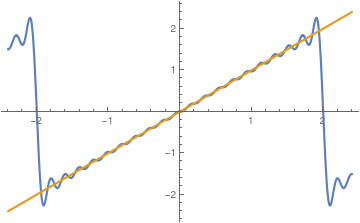
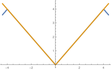
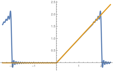
Example 4:
Let us consider a piecewise continuous function on interval [−π, π]:
Corollary:
If f(x) is a square integrable function (we abbreviate it as f∈𝔏²) then its Fourier coefficients tend to zero as n → ∞.
We have seen that under fairly general circumstances, Fourier expansions converge in the mean to the functions that gave rise to them. However, for many purposes, convergence in 𝔏² sense it is not sufficiently strong. Instead, we need either pointwise convergence or uniform convergence,
Fourier coefficients can be estimated with the aid of
the Bessel inequality:
Riesz--Fischer Theorem:
Suppose { bn }n = -∞∞ is a sequence of complex numbers with \( \sum_{n=-\infty}^{\infty} \left\vert b_n \right\vert^2 < \infty . \) Then there is a unique periodic function f ∈ 𝔏²(-π,π) such that \( b_n = c_n (f) = \frac{1}{2\pi} \,\int_{-\pi}^{\pi} f(x)\, e^{-{\bf j} nx} \,{\text d}x . \)
Example 7:
Consider an integrable function on [0, 1] with infinitely
many discontinuities is given by
\[
f(x) = \begin{cases}
1 , & \ \mbox{ if } \ 1/\left( n+1 \right) < x \le 1/n \ \mbox{ and $n$ is odd}, \\
0, & \ \mbox{ if } \ 1/\left( n+1 \right) < x \le 1/n \ \mbox{ and $n$ is even}, \\
0, & \ \mbox{ if } \ x = 0.
\end{cases}
\]
The function f is discontinuous
when x = 1/n and at x = 0.
■
Antonov, N.Y., Convergence of Fourier series, East Journal on Approximations, 1996,, 2, pp. 187--196.
du Bois-Reymond, P., Ueber die fourierschen reihen,
Königliche Gesellschaft der Wissenschaften zu Göttingen,
1873, Vol. 21, pp. 571--582.
Hunt, R.A., On the convergence of Fourier series,
Proc. Conf. Orthogonal Expansions and their Continuous Analogues, Southern Illinois Univ. Press (1968) pp. 234–255.
Kolmogorov, A., Une serie de Fourier--Lebesgue divergente presque partout, Fundamenta Mathematicae, 1923, 4, 324--328.
Konyagin, S.V., On divergence of trigonometric Fourier series, Comptes Rendus de l'Académie des Sciences - Series I - Mathematics, 1999, Vol. 329, pp.693--697.
Konyagin, S.V., On everywhere divergence of trigonometric Fourier series, Sb. Math. 191 (1), 97–120 (2000) [transl. from Математический сборник, 2000, 191, No. 1, pp. 103–126].
Körner, T.W., Fourier Analysis, Cambridge University Press, Great Britain, 1989.
Lacey, M. and Thiele, C., (2000), "A proof of boundedness of the Carleson operator", Mathematical Research Letters, 2000, Vol. 7 (4), pp. 361–370.
Lacey, M. and Thiele, C., Carleson's theorem: proof, complements, variations, Publicacions Matemàtiques, 2004, Vol. 48 (2), pp. 251–307
Ul'yanov, P.L., Kolmogorov and divergent Fourier series, Uspekhi Mat Nauk, 1983, Vol. 38, No. 4, 51--90; Russian math Surveys, 1983, 38, No. 4, pp. 57--100.
Return to Mathematica page
Return to the main page (APMA0340)
Return to the Part 1 Matrix Algebra
Return to the Part 2 Linear Systems of Ordinary Differential Equations
Return to the Part 3 Non-linear Systems of Ordinary Differential Equations
Return to the Part 4 Numerical Methods
Return to the Part 5 Fourier Series
Return to the Part 6 Partial Differential Equations