The Fokas method, or unified transform, is an algorithmic procedure for analyzing initial boundary value problems for linear partial differential equations and for an important class of nonlinear PDEs belonging to the so-called integrable systems. It is named after the Greek mathematician Athanassios S. Fokas (born in 1952), who introduced it in the late Nineties. The idea of the method was inspired by the 1994 article by Fokas and Gelfand.
The unified transform method can be considered as the analogue of Green’s function approach, but now it is formulated in the complex Fourier plane instead of the physical plane. It employs a global relation formulated in the Fourier plane which couples the initial and boundary data.
Certain nonlinear evolution PDEs, called integrable, can be formulated as the compatibility condition of two linear eigenvalue equations (Lax pairs). This technique is known as known as the
inverse scattering transform method. It has been emphasized by Fokas and Gelfand that this method is based on a deeper form of separation of variables. Indeed, the spectral analysis of the t-independent part of the Lax pair yields an appropriate nonlinear Fourier transform pair, whereas the t-dependent part of the Lax pair yields the time evolution of the nonlinear Fourier data. In this sense, despite the fact that the inverse scattering transform is applicable to nonlinear PDEs, this method still follows the logic of separation of variables by deriving a nonlinear Fourier transform pair.
Return to computing page for the first course APMA0330
Return to computing page for the second course APMA0340
Return to Mathematica tutorial for the first course APMA0330
Return to Mathematica tutorial for the second course APMA0340
Return to the main page for the first course APMA0330
Return to the main page for the second course APMA0340
Return to Part VI of the course APMA0340
Introduction to Linear Algebra with Mathematica
Previously, we discussed the separation of variables method that can be applied to certain classes of linear partial differential equations (PDEs for short). However, this method has serious limitations because not every linear PDE lends itself to separation of variables. Also it requires the given domain, the PDE, and the boundary conditions to be separable as well.
Success of the separation of variables method is based on having the spectral representation of a part of the differential operator in one variable. This means that this part can be represented by multiplication under a suitable transformation. In particular, the Laplace transform is a spectral representation of the derivative operator \( \texttt{D} = {\text d}/{\text d}t \) on the space of functions C¹[0,∞) vanishing at the origin and growing at infinity no faster than an exponential function. On the other hand, the Fourier transform is a spectral representation of the differential operator \( {\bf j}\,\partial /\partial x \) on the space of absolutely integrable functions on ℝ (this space is usually denoted by 𝔏) that approach zero at infinity.
Furthermore, separation of variables expresses the solution as either an integral or a series, neither of which are uniformly convergent on the boundary of the domain (for nonvanishing boundary conditions), which renders such expressions problematic for numerical computations. This reflects the facts that many initial boundary value problems (IBVP for short) for PDEs are not well-posed despite that they have unique solutions. For example, determination of the inverse Laplace or Fourier transforms are not well-posed problems.
The method, which was introduced in Fokas’ 1997 article in the Proceedings of the Royal Society is based on two novel steps:(i) Derive an algebraic equation, named by Fokas the global relation, which couples all boundary values. Some of these boundary values are prescribed as boundary conditions whereas the remaining are unknown functions. This equation involves an arbitrary complex parameter; hence, it is actually a family of equations. Exploring this fact, it turns out that it is possible to determine the unknown boundary values in terms of the given boundary data. This determination is often referred to as deriving the (generalized) Dirichlet to Neumann map. For evolution PDEs, and for elliptic PDEs in simple domains, this computation is analytic; for elliptic PDEs in complicated domains it can be achieved via highly efficient numerical algorithms. (ii) For evolution PDEs involving spatial derivatives of arbitrary order, and for elliptic PDEs formulated in simple domains, express the solution via an explicit integral representation involving contours in the complex plane.
History of the Fokas Method:
Certain nonlinear evolution PDEs in one spatial dimension, called integrable, can be formulated as the compatibility condition of two linear eigenvalue equations, called a Lax pair. This formulation gives rise to a method for solving the initial value problem of these equations, called the inverse scattering transform method. It was emphasized by Fokas and I.M. Gelfand (1913--2009) that this method is based on a deeper form of separation of variables. Indeed, the spectral analysis of the t-independent part of the Lax pair yields an appropriate nonlinear Fourier transform pair, whereas the t-dependent part of the Lax pair yields the time evolution of the nonlinear Fourier data. Indeed, if the nonlinearity is small, the above nonlinear Fourier transform pair reduces to the usual Fourier transform pair. Hence, the inverse scattering transform method and its extension to nonlinear evolution PDEs in two spatial dimensions which is called the d-bar method, provide the nonlinear analogues of the usual Fourier transform method in one and two spatial dimensions. It should be noted that despite the fact that the inverse scattering transform and the d-bar method are applicable to nonlinear PDEs, they still follow the logic of separation of variables: the nonlinear Fourier transform pair is obtained via the spectral analysis of the t-independent part of the Lax pair, which is analogous to obtaining the Fourier transform pair via the spectral analysis of the linear eigenvalue equation obtained via separation of variables.
In contrast to the reliance of the applicability of the linear and nonlinear Fourier transforms to evolution PDEs on separation of variables, the Fokas methods is based on the ‘synthesis of variables’: for evolution PDEs in one spatial variable x, the spectral analysis of the x-part of the Lax pair corresponds to deriving a transform in x, whereas the spectral analysis of the t-part of the Lax pair corresponds to deriving a transform in t; the Fokas method is based on the simultaneous spectral analysis of both parts of the Lax pair, and thus it corresponds to a ‘unified’ transform.
It is remarkable that the Fokas method was first discovered for integrable nonlinear PDEs. Indeed, although it was evident from the early 1970s that the inverse scattering provides a powerful method for solving the initial value problem of integrable PDEs, the question of extending the inverse scattering to boundary value problems remained open for more than two decades. The simplest such problem is the nonlinear Schrödinger equation (NLS for short) on the half-line with Dirichlet boundary conditions. A new methodology for solving this problem based on the formulation of a global relation and on the simultaneous spectra analysis of the Lax pair was presented in the
1997 paper of Fokas. Taking the linear limit of this formalism, Fokas was expecting to recover the representation obtained via the sine transform, since this is the classical x-transform used for the solution of the linearized version of the NLS; however, he obtained a completely new representation. In this way it was realized that a novel method for solving linear evolution PDEs was born.
The Fokas Method for Linear Evolution PDEs
The early implementation of the method to linear evolution PDEs was based on the Lax pair formulation. It was soon realized that it is possible to implement this method in a simpler way avoiding the Lax pair formalism. There is no doubt that for linear evolution PDEs the Fokas method provides a powerful approach going far beyond the existing methods. Furthermore, it has the important advantage that it leads to integral representations which can be computed easily via standard platforms. In more detail:
Any solution obtained via the usual transforms, such as the sine-transform, etc, has the major disadvantage that it is not uniformly convergent at the boundary of the given domain (except for the special case of homogeneous boundary conditions). Strangely, this pathology has not been mentioned in the standard textbooks. For example, in the case of the solution, u(x, t), of the heat equation with the Dirichlet boundary condition u(0, t) = f(t), obtained via the sine transform, if we attempt to verify this condition by letting x = 0 in the solution representation, we fail since sin 0 = 0. This implies that we cannot exchange the integral with the limit x → 0. In other
words, the solution representation is not uniformly convergent at x = 0, unless f(t) = 0.
This lack of uniform convergence makes the representations obtained via the usual transforms unsuitable for the numerical evaluation of the solution. Indeed, no numerical analyst uses such representations for the numerical evaluation of the solution.
Although there exists a systematic way for deriving the appropriate transform for a given boundary value problem, this approach is very complicated. Furthermore, for most problems this approach fails. For example, there does not exist an x-transform for the case where the second spatial derivative in the heat equation is replaced by a third derivative (this equation is physically significant, representing the linear limit of the celebrated Korteweg–de Vries (KdV) equation).
In contrast to these limitations, the Fokas method always constructs integral representations which are uniformly convergent at the boundary. Hence, these representations are most suitable for the numerical evaluation of the solution. Furthermore, the method is applicable to evolution PDEs with an arbitrary number of spatial derivatives.
The Fokas Method for Linear Elliptic PDEs
For elliptic PDEs in very simple domains the Fokas method is as effective as for evolution PDEs. Indeed, for such simple problems, some of which cannot be solved analytically by standard methods, it gives rise to explicit integral representations. Furthermore, just like the case of evolution PDEs, these explicit formulas give rise to simple and efficient numerical evaluations.
For elliptic PDEs in arbitrary convex polygonal domains, the utilization of the global relation gives rise to a novel spectral collocation method occurring in the Fourier space. Recent work
has extended the method, and has also demonstrated a number of its advantages, including the following: it avoids the computation of singular integrals encountered in traditional boundary based approaches, it is fast and easy to code up, it can be used for separable PDEs where no Green's function is known analytically, and it can be made to converge exponentially with the correct choice of basis functions.
Although the global relation is valid for non-convex domains, the collocation method becomes numerically unstable. This difficulty can easily be overcome by splitting up the domain into numerous convex regions (introducing fictitious, internal boundaries) and matching the solution and normal derivative across these internal boundaries. Importantly, such splitting also allows the extension of the method to exterior as well as to unbounded domains. In this connection it is noted that: (i) Complicated scattering problems, where the traditional Wiener-Hopf method fails, can be easily solved with the new method. (ii) A major advantage of the new collocation method is that the basis choice (such as Legendre
polynomials) can be flexibly extended by additional elements capable of capturing local properties of the solution along each boundary. This is useful when the solution has different scaling in different regions of the boundary, and it is particularly efficient for capturing singular behavior, for example, near sharp corners.
In a recent unexpected development, the method has been extended by M. J. Colbrook to elliptic PDEs with variable coefficient and curved boundaries.
Other Important Developments
Papers by hundreds of investigators have already been written analyzing various aspects of the method: from the works of A. Ashton on rigorous aspects of the method and its extension to elliptic PDEs in 3 dimensions, to a new methodology introduced by A. Himonas and D. Manzavinos for the use of the method for deriving rigorous well-posedness results for nonlinear evolution PDEs. Also, T. Ozsari and K. Kalimeris have shown that this method provides a new approach to solving important problems in the area of control. These developments justify the statement made in the early 2000s by I.M. Gelfand that “the Fokas method provides the most important development in the exact analysis of PDEs since the works of the classics”.
Short Curriculum Vitae of Athanassios Fokas
Fokas’ depth and versatility are evident from his seminal contributions in ten different areas: (i)symmetries and bi-Hamiltonian structures;(ii) Riemann--Hilbert and d-bar methods; (iii) Painlevé equations and Random matrices;(iv) the Fokas method;(v) inverse problems in nuclear medicine, including PET and SPECT;(vi) protein folding;(vii) algorithms in magneto-encephalography;(viii) asymptotic analysis to all orders of the Riemann-zeta function and a new approach to the Lindelöf hypothesis; (ix) important approximations of the two-body problem in general relativity;(x) predictive mathematical models for Covid-19. These works together with his forthcoming book “How we think, feel, and act; exploring cognition, computability, creativity, culture”, which elucidates unexpected connections in mathematics, physics, computer sciences, engineering, neuroscience, medicine, philosophy, painting, and music, justify Israel Gelfand’s statement in the early 2000s that “Fokas is a rare example of a scientist in the style of Renaissance”.
Fokas’s remarkably diverse contributions reflect his diverse background and interests. He has a BSc in Aeronautics from Imperial College (1975), a PhD in Applied Mathematics from Caltech (1979), and an MD from the School of Medicine of the University of Miami (1986).
Twenty years after his graduation from Imperial College he returned to his Alma mater where he occupied a chair in Applied Mathematics until 2002, when he was elected to the newly inaugurated chair of Nonlinear Mathematical Science at the University of Cambridge.
He has authored or co-authored five textbooks and has edited or co-edited eight books. His book with M. J. Ablowitz, Introduction and Applications of Complex Variables, Cambridge University Press, second edition (2003), is the standard book on the subject used in many universities; his book with A. R. Its and others, Painlevé Transcendents: A Riemann--Hilbert Approach, AMS (2006), is considered as the definitive monograph in this classical topic.
He has published more than 300 papers in journals and approximately 50 papers in various proceedings. He has an international patent in magneto-electroencephalography. He has been included by ISI in the list of highly cited researchers in Mathematics.
His research has been funded by a variety of sources. In particular, he was supported from the Mathematical Section of the National Science Foundation of the USA in the period 1982-1995 and from the Mathematical Division of the Air Force Office of Scientific Research of USA in the period 1987-1995 (except for 1983-86 because of his medical studies). He has been supported continuously from the Engineering and Physical Sciences Research Council (EPSRC) since his return to the UK. In particular, for the period 2015--2020 he was fully supported via a prestigious Senior Fellowship. Also, for the period 2016--2020 he wass a co-investigator in the 2.5 million funding supporting the Center for Mathematical Imaging in Healthcare in the University of Cambridge.
He has given more than 350 talks in Congresses, International Conferences and Workshops and Colloquia. He has also delivered many presentations for wide audiences on the relations between philosophy, mathematics, physics, medicine, neuroscience, music, and painting, in places including: the Athens Concert Hall, Cambridge, Harvard, Oxford, and Beijing (disambiguating Peking), the capital city of the People's Republic of China.
Fokas was a co-founder of the Journal of Nonlinear Sciences, and he is serving or has served in the editorial board of several journals, including Proceeding of the Royal Society, Selecta Mathematica, Nonlinearity, and Studies in Applied Mathematics.
Fokas received several distinctions. In 2000, the London Mathematical Society awarded him the Taylor Prize (this prize was awarded on the occasion of the millennium; a year earlier, the recipient of this prize was S. Hawking). In 2009 he was awarded a Guggenheim fellowship. He has been awarded the Ariston Prize of Sciences of the Academy of Athens (the most prestigious prize of the Academy awarded every four years), as well as the Excellence Prize of the Bodossaki foundation jointly with D. Christodoulou. His biomedical contributions were recently recognized with his election to the American Institute of Medical and Biological Engineering. He is the only applied mathematician to have been elected a full member of the historic Academy of Athens. Also, he has been decorated as the Commander of the order of Phoenix by the President of the Hellenic Republic. He has received honorary degrees from seven universities. He is a Professorial fellow of Clare Hall Cambridge, as well as a member of the European Academy of Sciences.
Short Historical Note about Athanassios Fokas and his collaborators
There is a particular class of nonlinear evolution PDEs called integrable. These equations, which include the Korteweg–de Vries (KdV) equation and Nonlinear Schrödinger equation (NLS), have a variety of remarkable properties. These include the possession of infinitely many symmetries, which can be constructed recursively via the recursion operator, first obtained by Peter Olver in connection with the KdV. Moreover, Franco Magri established that they admit a bi-Hamiltonian formulation; namely, they can be written as a Hamiltonian system via two different Hamiltonians. Actually, there is a beautiful relation between the recursion operator and the two Hamiltonians. This was established independently by Israel Gelfand (1913--2009), his student Irene Dorfman (--1994), as well as by Athanassios Fokas (born June 30, 1952, island of Kafalonia, Greece) and Benno Fuchssteiner.
Israel Gelfand was born to Jewish parents in the small town of Okny to the north of Odessa, the Russian empire. I.
Gelfand (1913--2009) went to Moscow at the age of 16. There he took on a variety of different jobs such as door keeper at the Lenin library---this was the place where he met Andrew Kolmogorov (1903--1987). He was the person who helped Gelfand to be admitted in 1930 directly into graduate school at Moscow State University before completing his secondary education. Gelfand completed his ordinary doctorate in 1935 (without having a college diploma) and then a higher doctor of mathematics degree in 1940. By the way, Kolmogorov was forced to work as a conductor before entering Moscow University because of his aristocratic heritage.
Dr. Gelfand did not achieve fame from attacking and solving famous, intractable problems (as, for example, his adviser Andrew Kolmogorov who solved several Hilbert's problems). Instead, he was a pioneer in introducing mathematical fields, laying the foundation and creating tools for others to use. Gelfand discovered a special algorithm (he called it "progonka") for solving numerically algebraic system of equations with a tri-diagonal matrix, but refused to accept his recognition because he thought it was easy. This algorithm is known now as FEBS (first elimination, back substitution) or the Thomas algorithm (1949, Elliptic Problems in Linear Differential Equations over a Network, Watson Sci. Comput. Lab Report, Columbia University, New York).
Gelfand's seminar series, run independently of the university and open to anybody, ran for nearly 50 years and is famous throughout the mathematical community. Israel always tried to make his seminars interactive to involve the audience into discussion so no one left without understanding the topic.
Gelfand was very impressed by the bi-Hamiltonian property: he announced in a conference in Russia in 1979 that the ‘essence of integrability is the existence of two Hamiltonians’. However, despite the efforts of many distinguished researchers, neither a recursion operator nor a bi-Hamiltonian formulation could be found for integrable nonlinear evolution equations in two-spatial dimensions. The distinguished Russian mathematical physicist Vladimir Zakharov together with Boris Konopelchenko proved that such structures, of a general type naturally motivated from the results in one spatial dimension, did not exist (see their article). In the early 1980’s, after their success with Mark Ablowitz in extending the inverse scattering formalism for the solution of integrable PDEs from one to two spatial dimensions, Fokas also tried unsuccessfully to construct recursion operators in two spatial dimensions. Actually, when Athanassios left mathematics to study medicine in 1983, there were two important problems in the theory of integrable systems: the solution of boundary value problems for evolution equations in one spatial dimension, and the construction of a bi-Hamiltonian formulation in two spatial dimensions. As soon as Athanassios returned to mathematics, he solved together with Paolo Santini the latter problem introducing a novel type of mathematical structures (called operands).
In April of 1987, Fokas visited Moscow and he called Gelfand to tell him that he was right: since the bi-Hamilton formulation does exist for integrable PDEs both in one and two spacial dimensions, it is indeed a fundamental property of integrability. Gelfand agreed to meet Athanassios in his apartment in Moscow, where Fokas went together with the late distinguished mathematician Genadi Henkin and his son Roman Novikov. It was a very warm meeting. Athanassios promised to send him certain books in neuroscience that he requested, and to be in touch.
Around that time, Fokas decided to edit a book, Important Developments in Soliton Theory, in order to announce his return to mathematics from medicine. His friend Vladimir Zakharov (born August 1, 1939) agreed to be a co-editor. The idea was to invite as contributors the most distinguished researches in the area of integrable systems. For the topic of the bi-Hamiltonian formulation he decided with Vladimir that the best choice would be Gelfand. But when Fokas contacted him with this request, he suggested (knowing of their recent work on two dimensions) that they write it jointly. Meanwhile, Gelfand had immigrated to the USA. Thus, there began their collaboration which led to a deep friendship. In particular, Israel together with his wife and daughter (both named Tanya) spent a month in the Greek island of Kafalonia, as Fokas' guests, in the summer of 1991.
A.Fokas recalls:
I will never forget the day they arrived in Athens: after meeting them in the airport we went to a hotel where they laid down to rest, exhausted from my trip from Kafalonia to Athens and, more importantly, from the stress of making sure all arrangements were in place. But, there appeared Gelfand, who instead of resting after the long flight from the States, wanted to do mathematics! While we were in Kafalonia, another close friend, the ‘father of integrable systems’ Martin Kruskal (1925--2006), called me from Patras, Greece, asking if he could come to Kefalonia. Martin was often quite aggressive. However, in front of Israel he was like a schoolboy. Every night, we ate together, Israel with his wife and daughter, myself with my former wife Allison (after putting our one-year old son Alexander to sleep) and Martin. There were many fascinating stories; I will only mention one: one night, Martin said to Israel: “you must be very content with your great double life as a mathematician and a biologist. Have you thought what you would want to be if you were not involved with mathematics and biology?” Gelfand did not hesitate at all; he immediately answered, “a conductor”. Allison was very surprised: a few years earlier, she had asked me the same question and I had given the same answer (without any clue that Gelfand's adviser, A. Kolmogorov, actually worked as a conductor).
During our time together in Kefalonia, we understood with Gelfand that the Riemann-Hilbert and d-bar formalism provide a unified approach to linear and integrable nonlinear PDEs. Indeed, these mathematical tools can be used to construct the classical Fourier transform in one and two spatial dimensions, which can be used for the solution of linear PDEs. Also, the tools above can be employed for the construction of nonlinear versions of the Fourier transform in one and two dimensions that are needed for the integration of the integrable nonlinear versions of certain linear PDEs. Furthermore, our work led to the introduction of a new approach for constructing transforms, which was used by Roman Novikov (more than a decade later) for the solution of an open problem in the imaging technique of SPECT. Our time in Kefalonia sealed our friendship. The evening before flying back to the USA, Israel told me: “I do not know what I will to do without you”. Israel’s impact on my life has been immense.
I have been fortunate to have worked and co-authored papers with several distinguished mathematicians, including Gelfand, Zakharov, and Joe Keller. Kruskal, was certainly the most brilliant and the only person in my entire life that for several years gave me an inferiority complex.
It is not known to most mathematicians that Gelfand made important contributions in biology, especially deciphering some of the functions of the cerebellum. Interestingly, he never used mathematics in his biological work. It is not known that one of the areas that we worked together was in protein folding.
★
This section presents an introduction to the Fokas method or unified transform method that can handle systems of partial differential equations with two independent variables. Note that it is not clear how to expand the method for the case of more than two independent variables. For our presentation of the Fokas method, we choose the heat transfer (also known as diffusion) equation with constant coefficients
for two reasons.
First of all, it is a very simple partial differential equation (PDE) and one expects that all computations could be accomplished explicitly. Second, this equation can be considered as a typical PDE that involves two distinct independent variables: one is a time variable (which we naturally denote by t) and another one is a spatial variable (for which we use x). Accordingly, the heat equation involves two unbounded differential operators with known spectral decompositions for each of them.
Given the initial data u(x,0) = f(x), we arrive at the initial value problem:
\begin{align*}
&\mbox{Heat conduction equation:} \qquad &u_t &= \alpha\,u_{xx} \qquad\mbox{for } -\infty < x < \infty \mbox{ and } t > 0, \\
&\mbox{Initial condition:} \qquad &u(x,0) &= f(x) , \qquad -\infty < x < \infty .
\end{align*}
Since the domain for the spatial variable x is unbounded, we need to impose some conditions on the behavior of the solution u(x,t) and the initial temperature f(x) at infinity. It is natural to assume that these functions (f(x), u(x,t) and its derivatives ut, ux, and uxx) become zero as x → ±∞. However, for our purposes, we need also to assume that these functions decay at infinity fast enough to guarantee that all functions are square integrable (so they belong to the space 𝔏²). This condition, which we call the regularity condition, is needed to make a corresponding initial value problem well-posed. Note that for wave propagation problems, this condition is called the radiation condition and it is not as simple as our regularity condition for heat conduction equations.
Using the derivative operators \( \texttt{D} = \partial /\partial t \) for the time derivative and ∂x = ∂/∂x for the spatial derivative, we introduce the differential operator corresponding to the heat conduction equation:
We know from Chapter 5 that the Fourier transform (since there is no universal abbreviation for the Fourier transform, we recall the three possible distinct notations) is defined as the improper integral
The Fourier transformation
gives the spectral representation of the derivative operator j ∂x. It means that the Fourier transformation represents this differential operator as a multiplication operator:
It was previously shown in the opening section that
the solution of the corresponding initial value problem can be expressed through the Fourier transform of the initial data as
As it is seen from the preceding formulas, the solution is represented as an improper integral (in the Cauchy principle value sense) over either a horizontal axis (Fourier) or a vertical line (Laplace). It is known that the Laplace transformation is a particular case of the Fourier transform applied to functions that are identically zero for negative t. We will see shortly that
the Fourier integral is preferable over the Laplace counterpart because the former is more flexible in defining functions for negative argument not necessarily identically vanishing.
It can be shown that the Bromwich integral can be transformed into the Fourier one by changing variables and using the Cauchy integral theorem and Jordan's lemma. For completeness, we present one of its versions that is more suitable for Fourier integration.
Jordan's Lemma:
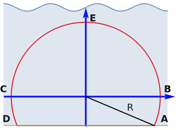
Let R be a positive number and 𝑎 be a real number with |𝑎| < R. Let
\[
C_R = \left\{ z \in \mathbb{C} \, : \, |z| = R \quad\mbox{and} \quad \Im z \ge -a \right\}
\]
be a part of the circle of radius R in the upper half of the complex plane ℂ bounded by the horizontal line Im z = −𝑎; this part of the plane ℂ is denoted by \( S_a = \left\{ z \in \mathbb{C} \, : \, \Im z \ge -a \right\} . \) Let f be a continuous function in the upper part of the plane S𝑎 that tends to zero uniformly as R → ∞. That is, for any positive ε, there exists K ≥ R such that z ∈ S𝑎 and |z| > K implies that \( | f(z) | < \varepsilon . \) Then for any positive m, we have
Let \( z = x+ {\bf j}\,y = R\, e^{{\bf j}\,\theta} \) be a complex number and \( \quad M_R = \max_{C_R} \left\vert f(z) \right\vert , \quad \alpha = \arcsin \frac{a}{R} . \)
According to conditions of Jordan's lemma, MR → 0 as R → ∞; also α tends to zero and the product
α R → 𝑎 as R → ∞. For 𝑎 > 0, we have
\( \left\vert e^{{\bf j}mz} \right\vert = e^{-my} \le e^{am} \)
on arcs AB and CD. Hence,
It can be shown that \( \displaystyle \sin\phi \ge \frac{2}{\pi}\,\phi \) because the derivative
\( \displaystyle \frac{\text d}{{\text d}\phi} \left( \frac{\sin\phi}{\phi} \right) = \frac{\cos\phi}{\phi^2} \left( \phi - \tan\phi \right) \) is negative on the interval (0, π/2).
So we conclude that along the arc BE
tends to zero as R → ∞, as well as a similar integral over the arc EC.
▣
Notes: Marie Ennemond Camille Jordan (1838--1922) was a French mathematician who published the lemma that now bears his name in very influential journal, Cours d'analyse (Gauthier-Villars, 1909).
When m < 0, the lemma is still valid but for a family of circles in the domain ℑz ≤ 𝑎.
Jordan's lemma: For a family of parts of circles in the domain ℜp ≤ 𝑎, we have
\[
\lim_{R\to \infty} \int_{C_R} f(-{\bf j}p)\, e^{mp} {\text d}p = 0 , \qquad C_R \in \Re p \le a.
\]
Here CR is a part of a circle of radius R in the half plane ℜp ≤ 𝑎.
■
Green’s theorem: Let R be the region bounded by a positively oriented (if it is traced out in a counter-clockwise direction the domain R is on the left), piecewise smooth, simple closed curve ∂R. If P and Q are functions of (x, y) defined on an open region containing R and having continuous partial derivatives there, then
where the path of integration along ∂R is counterclockwise.
▣
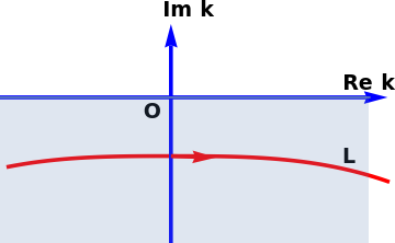
However, once we try to apply one of these transforms (either Fourier or Laplace) to solve some initial boundary value problems, we immediately see an obstacle of interference of the spectral representation with the boundary conditions---they cannot be incorporated into these integral transformations. The main achievement of A. Fokas is the observation that solutions to a wide class of the initial boundary value problems with two independent variables can be still represented in the form similar to the Fourier transform
where L is an appropriate contour on the complex plane ℂ, ω(k) is the dispersion relation, and ρ is some analytic function of a complex variable k. The preceding integral formula gives the complete spectral decomposition of the given initial boundary value problem in the sense that the operator generated by the differential equation subject to appropriate initial and boundary conditions becomes a multiplication in the Fourier space.
There are some advantages of using the Fokas method.
The integral form of the solution guarantees that the differential equation is satisfied.
The entire problem in two independent variables is transformed into finding the function ρ(k) of a single variable k and the one-dimensional contour of integration L in the complex plane ℂ.
The Fokas method allows one to determine in a straight forward way when the boundary conditions make the corresponding problem well-posed; in some sense, the obtained conditions generalize the well-known Shapiro--Lopatinski conditions for elliptic equations.
Upon deforming the line of integration L, the corresponding integral could be made more computationally friendly.
The unified explicit integral formula for the solution is more suitable for asymptotic analysis, which is very important in applications.
The unified transform method is the actual realization of the
Fundamental Principle that was formulated in 1960 by the American mathematician
Leon Ehrenpreis (1930--2010) with a mistake that was corrected by
the Russian mathematician
Victor Pavlovich Palamodov (born in 1938). We formulate the
Ehrenpreis Fundamental Principle suitable for our purposes.
Ehrenpreis--Palamodov Theorem:
The solutions of a linear system of PDEs with constant coefficients can be represented in terms of certain integrals.
The starting point of the Fokas method is to write the PDE as a one-parameter family of equations formulated in a divergence form---this allows one to consider the independent variables together. In this sense, the method is based on the “synthesis” as opposed to the “separation” of variables.
We illustrate the Fokas method (or unified transform) by considering the heat
equation on the quarter plane ℝ²+ (0 < x, t < ∞) with three types of boundary conditions: Dirichlet, Neumann, and mixed. So we will deal with the initial boundary value problem (IBVP):
where R = { 0 < x, t < ∞} = (0, ∞) × (0, ∞).
We can obtain different boundary conditions upon choosing particular numerical values of parameters 𝑎 and b. Note that the cases when 𝑎 = 0 or b = 0 correspond to well-known Neumann or Dirichlet boundary conditions, respectively; they will be considered separately.
The initial step in the Fokas method is to apply the standard Fourier
transformation to the differential equation in order to determine the dispersion relation. It is equivalent to seeking a solution in the form \( u(x,t) = e^{-\omega (k)\,t - {\bf j} kx} . \) This step was accomplished previously in section iv and we know that ω(k) = α k².
Next, we multiply the heat differential equation by \( e^{\omega (k)\,t + {\bf j} kx} , \) the reciprocal of the exponential function in the Ehrenpreis integral formula (Fourier.4), and rearrange them into the divergent form using the product derivative rule. This yields:
\[
e^{\omega (k)\, t + {\bf j}kx} u_t = \left( e^{\omega (k)\, t + {\bf j}kx} u \right)_t - \omega (k)\, e^{\omega (k)\, t + {\bf j}kx} u , \qquad \omega (k) = \alpha\, k^2 ,
\]
and
\begin{align*}
e^{\omega (k)\, t + {\bf j}kx} u_{xx}&= \left( e^{\omega (k)\, t + {\bf j}kx} u_x \right)_{x} - {\bf j}k\, e^{\omega (k)\, t + {\bf j}kx} u_{x}
\\
&= \left( e^{\omega (k)\, t + {\bf j}kx} u_x \right)_{x} - {\bf j}k \left( e^{\omega (k)\, t + {\bf j}kx} u_x \right)
\\
&= \left( e^{\omega (k)\, t + {\bf j}kx} u_x \right)_{x} - {\bf j}k \left( e^{\omega (k)\, t + {\bf j}kx} u \right)_{x} - k^2 e^{\omega (k)\, t + {\bf j}kx} u .
\end{align*}
Then the heat equation ut = α uxx will be equivalent (upon multiplication by the non-zero exponential term \( e^{\omega (k)\,t + {\bf j} kx} \) ) to
\[
\left( e^{\alpha\,k^2\, t + {\bf j}kx} u \right)_t - \alpha\,k^2 e^{\alpha\,k^2\, t + {\bf j}kx} u = \alpha \left[ \left( e^{\alpha\,k^2\, t + {\bf j}kx} u_x \right)_{x} - {\bf j}k \left( e^{\alpha\,k^2\, t + {\bf j}kx} u \right)_{x} - k^2 e^{\alpha\,k^2\, t + {\bf j}kx} u \right]
\]
or upon cancellation of the common terms to
\[
\left( e^{\omega (k)\, t + {\bf j}kx} u \right)_t - \alpha \left( e^{\omega (k)\, t + {\bf j}kx} u_x \right)_{x} + \alpha {\bf j}k \left( e^{\omega (k)\, t + {\bf j}kx} u \right)_{x} = 0 , \quad \omega (k) = \alpha\,k^2 .
\]
The above equation written in a divergence form is called the
local relation
because it is held independently of the solution domain and the boundary conditions.
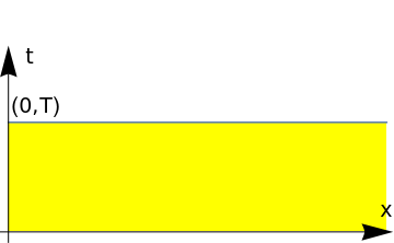
Further, we consider a truncated domain of integration
RT = { (x,t) : 0 < x < ∞, 0 < t < T }. for some positive real number T.
Now we integrate our local relation written in the divergence form over domain
RT:
\[
\int_{R_T} {\text d} S \left[ \left( e^{\alpha\,k^2\, t + {\bf j}kx} u \right)_t - \alpha \left( e^{\alpha\,k^2\, t + {\bf j}kx} u_x \right)_{x} + \alpha {\bf j}k \left( e^{\alpha\,k^2\, t + {\bf j}kx} u \right)_{x} \right] = 0 ,
\]
where dS is a surface element.
Then we apply
Green's theorem to the two-dimensional integral above that allows us to reduce it to integration over the one-dimensional boundary
∂RT of
RT = { 0 < x < ∞, 0 < t < T < ∞ }, oriented so that the domain RT is on the left when the boundary is traced.
Since the boundary ∂RT consists of three straight lines
t = 0, 0 < x < ∞,
t = T, 0 < x < ∞,
x = 0, 0 < t < T,
the last integral over the boundary becomes
\[
- \int_0^{\infty} e^{{\bf j}kx} u(x,0) \,{\text d} x + \int_0^{\infty} e^{\omega (k)\, T + {\bf j}kx} u(x,T) \,{\text d} x + \int_0^T \left( - \alpha\,e^{\omega (k)\, t} \, u_x (0,t) + \alpha\,{\bf j}\,k\, e^{\omega (k)\, t} \, u (0,t) \right) {\text d} t =0 ,
\]
where ω(k) = α k² is the dispersion relation.
This equation is referred to as the global relation for the heat conduction equation on the half line because it connects the initial condition and the boundary data with the value of the (unknown yet) function u( x, T) at arbitrary T. The global relation is valid for any t ∈ (0,T). Replacing T by t, we obtain
Multiplying the preceding equation by
\( e^{-\omega (k)\, t} = e^{-\alpha\,k^2\, t} \ne 0 \) and isolating the corresponding integral, we get a relation that is equivalent to the
global relation:
The integral in the left-hand side resembles the Fourier transform, but the integral's lower limit is 0 and not −∞. To make it a full Fourier transformation, we extend the (still unknown) function u(x,t) for negative x:
\[
U(x,t) = \begin{cases} u(x,t), & \ \mbox{ for } \ x \ge 0,
\\
u_{-} (x,t) , & \ \mbox{ for } \ x < 0 , \end{cases}
\]
where u− is some integrable function that can be chosen to be arbitrary, for instance, identically zero. However, we will choose this function wisely depending on the boundary conditions. Determination of u− is essential when the Fourier transformation method is used directly. So
If the integrals on the right-hand side can be transformed to the form containing only the given initial condition and the boundary data, then the given initial boundary value problem is well-posed. The presence of unknown boundary conditions hints at an ill-posed problem. The following examples demonstrate how the dispersion relation can be used to determine the unknown function u-(x, t) in order to eliminate all unknown data in the integrals of Eq.(Fokas.3).
Diffusion equation with the Dirichlet boundary condition
We consider the heat conduction equation with the Dirichlet boundary condition:
The objective of the unified transform method is to show that the integral J(x,t) can be expressed through known data for positive arguments x,t.
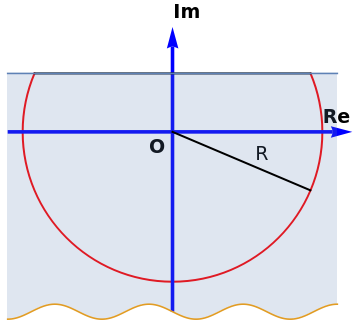
Clarification:
The integrals over the Fourier parameter k converge uniformly in the domain T = t - τ ≥ ε > 0 due to fast exponential decay of the integrand. However, when T becomes small and close to zero, we lose uniform convergence and it forces us to find another way for their evaluations.
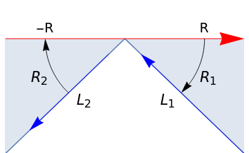
In order to achieve it, we remark that the integrand is an analytic function in variable k, and we need to consider the following auxiliary integral
Although the integration in the above integral is over a real axis, the terms are holomorphic functions and we can analytically continue the integrand into the lower-half of the complex k-plane due to the exponential decay of its integrand. Indeed, if k = ξ + jη, where j is the unit vector in the positive vertical direction on the complex k-plane ℂ, then the real parts are
along the contour as shown in the picture above. Since the integrals over circular arcs R1 and R2 tend to zero as the radius R grows according to Jordan's lemma, we claim that integral I is equivalent to the sum of two integrals
The expression for u(x,t) obtained from the global relation still does not present a solution because it depends on boundary data we have not prescribed through ux(0,t) and u−(x,t). To resolve this problem, we use the global relation again. So we invoke it in the original form:
we replace x by -x in the integral over k, which is equivalent to switching to the negative k (see formula (Fourier.3) for the Fourier transform above):
Therefore, the dispersion relation ω(k) = α k² for the heat equation, which is invariant for negative translations, dictates the extension of the unknown function u(x, t) for negative x, independently of how one defines the function u−. Even if you initially decided to set u− identically zero, the formula for U(-x,t) identifies the function for x < 0. This means that the mathematics involved decides how to extend the function u(x, t) for negative x, but not you!
Subtracting the formula for U(-x,t) from the expression for U(x,t), we obtain
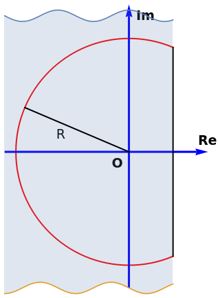
that does not converge uniformly: when τ is close to t, the integral diverges. To change the order of integration, we transfer the integral over Fourier parameter k into the complex plane ℂ and choose the contour of integration into another path to guarantee fast exponential decrease of the integrand.
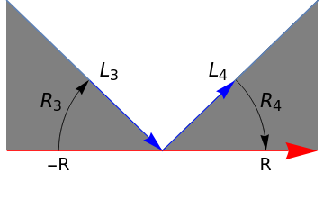
Again, we consider the following auxiliary integral for T = t - τ ≥ 0:
The corresponding domain of convergence is denoted in gray color in the figure above. Then transferring the integral from the real axis into the lines L3 and L4, we get
We show how A. Fokas solved this problem without actual continuation for negative x. His idea is based on utilization of the symmetry of the dispersion relation. So we rewrite the global relation (Fokas.1) for -k, and obtain
If we extend our function u(x, t) in the odd way along the x-axis and set \( \displaystyle u_{-} (x,t) = - u(-x,t) , \) then the two integrals on the left-hand side cancel each other and we obtain one equation for determination of the Neumann boundary data:
Substitution of the left-hand side integral into the global relation (Fokas.1) gives the expression for the solution without Neumann boundary data. This is exactly Eq.(Fokas.4).
■
\[
U(x,t) = \begin{cases} u(x,t), & \ \mbox{ for } \ x \ge 0,
\\
u_{-} (x,t) , & \ \mbox{ for } \ x < 0 , \end{cases}
\]
is a continuation of u(x,t) for negative x, so the function u−(x,t) is still unknown.
All other terms on the right-hand side are known except the integral containing u(0,t):
If we extend our function u(x, t) in the even way along the x-axis and set \( \displaystyle u_{-} (x,t) = u(-x,t) , \) then the two integrals on the left-hand side cancel each other and we obtain one equation for determination of the Dirichlet boundary data:
Substitution of the left-hand side integral into the global relation (Fokas.1) gives the expression for the solution without Dirichlet boundary data. This is exactly Eq.(Fokas.5).
■
Diffusion equation with the mixed boundary condition
We consider the heat
equation on the half line with the boundary conditions of the third kind:
We assume that the positive coefficients 𝑎 = 1 (without any loss of generality) and b are known.
Using the boundary condition u(0,t) = g(t) + bux(0,t), we have from the global relation (Fokas.1) that
Then we rewrite this equation for negative k using the property of the dispersion relation to be invariant under negative invension: \( \displaystyle \omega (k) = \omega (-k) , \) where ω(k) = α k². This yields
Substituting the expression for integral containing ux(0, τ) into Eq.(Fokas.6), we obtain
\begin{align*}
\int_0^{\infty} e^{{\bf j}kx} u(x,t) \,{\text d} x &= \int_0^{\infty} e^{{\bf j}kx - \alpha\,k^2\, t} f(x) \,{\text d} x - {\bf j}\,k\, \alpha \int_0^t e^{- \alpha\,k^2\left( t- \tau \right)} g (\tau )\, {\text d} \tau
\\
&\quad + \frac{1 - {\bf j}\,k\, b }{1 + {\bf j}\,k\, b }\, \int_0^{\infty} e^{-{\bf j}kx} u(x,t) \,{\text d} x - \frac{1 - {\bf j}\,k\, b }{1 + {\bf j}\,k\, b }\, \int_0^{\infty} e^{-{\bf j}kx - \alpha\,k^2\, t} f(x) \,{\text d} x - {\bf j}\,k\, \alpha \,\frac{1 - {\bf j}\,k\, b }{1 + {\bf j}\,k\, b }\, \int_0^t e^{- \alpha\,k^2\left( t- \tau \right)} g (\tau )\, {\text d} \tau .
\end{align*}
We group similar terms together and simplify
\begin{align*}
\int_0^{\infty} u(x,t) \left[ e^{{\bf j}kx} - \frac{1 - {\bf j}\,k\, b }{1 + {\bf j}\,k\, b }\, e^{-{\bf j}kx} \right] {\text d} x &=
e^{- \alpha\,k^2\, t} \int_0^{\infty} f(x) \,{\text d} x \left[ e^{{\bf j}kx} - \frac{1 - {\bf j}\,k\, b }{1 + {\bf j}\,k\, b }\, e^{-{\bf j}kx} \right]
\\
&\quad - \frac{2 {\bf j}\,k\, \alpha }{1 + {\bf j}\,k\, b }\, \int_0^t e^{- \alpha\,k^2\left( t- \tau \right)} g (\tau )\, {\text d} \tau .
\end{align*}
In order to solve the given initial boundary value problem (IBVP for short) with the mixed boundary condition, we extend the (unknown yet) function u(x,t) for negative x:
\[
U(x,t) = \begin{cases}
u(x,t), & \ \mbox{ for } x\ge 0, \\
u_{-} (x,t), & \ \mbox{ for } x < 0.
\end{cases}
\]
Then the previous expression can be written as
\begin{align*}
\int_{-\infty}^{\infty} U(x,t) \, e^{{\bf j}kx} {\text d} x &=
\int_{-\infty}^{0} u_{-} (x,t) e^{{\bf j}kx} {\text d} x + \int_{0}^{\infty} u(x,t) \, e^{-{\bf j}kx} \,\frac{1 - {\bf j}\,k\, b }{1 + {\bf j}\,k\, b }\, {\text d} x
\\
&\quad + e^{- \alpha\,k^2\, t} \int_0^{\infty} f(x) \,{\text d} x \left[ e^{{\bf j}kx} - \frac{1 - {\bf j}\,k\, b }{1 + {\bf j}\,k\, b }\, e^{-{\bf j}kx} \right]
- \frac{2 {\bf j}\,k\, \alpha }{1 + {\bf j}\,k\, b }\, \int_0^t e^{- \alpha\,k^2\left( t- \tau \right)} g (\tau )\, {\text d} \tau .
\end{align*}
The left-hand side is the Fourier transform of the function U(x, t) with respect to the spatial variable x, so
is the Fourier transformation of the unknown function U(x,t) with respect to spatial variable x. Before taking the inverse Fourier transform, let us consider the auxiliary integral
So the half-Fouirer transform of the unknown function u−(−ξ, t) is determined through the half-Fourier transform of the function u(ξ, t) multiplied by the ratio \( \displaystyle \frac{1 - {\bf j}\,k\, b }{1 + {\bf j}\,k\, b } . \)
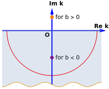
This is possible only when all singular points for their half-Fourier transforms lay in the lower half-space Im k < 0 where Jordan's lemma is valid.
Figure 7: Jordan region for the auxiliary integral J(k, t) and possible singularity kb.
Mathematica code
The relation (Fokas.9) defines the function u−(-ξ, t) via its half-Fourier transformation. The Dirichlet boundary condition is obtained by taking the limit (from the right) as b → 0+ in Eq.(Fokas.9), which is equivalent to the requirement that u(x, t) be extended for negative x in the odd way (u(−x, t) = −u(x, t)). Similarly, for the Neumann boundary condition we obtain the even extension (u(−x, t) = u(x, t)) when b → ∞. However, when b ≠ 0, this extension becomes more complicated and it should follow Eq.(Fokas.9).
It is well-known that the case b < 0 has no physical meaning as the temperature cannot flow from lower to higher values. This fact is reflected by Eq.(Fokas.9) because application of the inverse Fourier transformation requires the inclusion of a term due to the residue at k = j/b in the lower half complex plane Im k < 0. As a result, we will get an additional term corresponding to a source of energy with an exponential term that does not tend to zero as t → +∞, which violates the regularity condition:
Applying the Fourier transformation to the given differential equation ut + α uxxx = 0, we get the dispersion relation ω(k) = −jαk³, with j being a unit vector in the positive vertical direction on the complex plane ℂ, so j² = −1. Hence the solution of the given initial boundary value problem (IBVP for short) can be represented in the Ehrenpreis form:
where L is a contour obtained by continuously deforming the Fourier line of integration in the complex k-plane.
This means that the integral \eqref{Eq3PDE.1} satisfies the third order partial differential equation ut + α uxxx = 0 for any square integrable smooth function ρ(k) ∈ 𝔏²(L) such that k³ρ(k) ∈ 𝔏²(L).
Following A.Fokas, we will show how to determine function ρ(k) and the contour L so that integral \eqref{Eq3PDE.1} also satisfies the initial (u(x, 0) = f) and boundary (u(0, x) = g) conditions. Although Eq.\eqref{Eq3PDE.1} resembles the inverse Fourier transform, the path of integration L cannot be chosen as the real axis (-∞, ∞) used in the Fourier transformation.
We multiply the given differential equation by the reciprocal of the exponential function in the Ehrenpreis integral formula:
\[
e^{-\omega (k)\, t + {\bf j}kx} u_t = e^{{\bf j}\alpha\,k^3\, t + {\bf j}kx} u_t = \left( e^{{\bf j}\alpha\,k^3\, t + {\bf j}kx} u \right)_t - {\bf j}\alpha\,k^3 e^{\alpha\,k^3\, t + {\bf j}kx} u ,
\]
and regroup terms in order to get a divergence form:
\begin{align*}
e^{{\bf j}\alpha\,k^3\, t + {\bf j}kx} u_{xxx} &= \left( e^{-\omega (k) \, t + {\bf j}kx} u_{xx} \right)_{x} - {\bf j}k\, e^{-\omega (k) \, t + {\bf j}kx} u_{xx}
\\
&= \left( e^{-\omega (k) \, t + {\bf j}kx} u_{xx} \right)_{x} - {\bf j}k \left( e^{-\omega (k) \, t + {\bf j}kx} u_x \right)_x - k^2 e^{-\omega (k) \, t + {\bf j}kx} u_x
\\
&= \left( e^{-\omega (k) \, t + {\bf j}kx} u_{xx} \right)_{x} - {\bf j}k \left( e^{- \omega (k) \, t + {\bf j}kx} u_x \right)_{x} - k^2 \left( e^{-\omega (k) \, t + {\bf j}kx} u \right)_{x} +{\bf j} k^3 e^{- \omega (k) \, t + {\bf j}kx} u .
\end{align*}
Then the given equation ut + α uxxx = 0 will be equivalent (upon multiplication by the non-zero exponential term \( e^{-\omega (k) \, t + {\bf j}kx} \) ) to
\[
\left( e^{-\omega (k) \, t + {\bf j}kx} u \right)_t - {\bf j} \alpha\,k^3 e^{- \omega (k) \, t + {\bf j}kx} u + \alpha \left[ \left( e^{- \omega (k) \, t + {\bf j}kx} u_{xx} \right)_{x} - {\bf j}k \left( e^{- \omega (k) \, t + {\bf j}kx} u_x \right)_{x} - k^2 \left( e^{- \omega (k) \, t + {\bf j}kx} u \right)_x + {\bf j} k^3 e^{{\bf j} \alpha\,k^3\, t + {\bf j}kx} u \right] = 0,
\]
or after cancellation of the common terms to
\begin{equation*}
\left( e^{-\omega (k)\, t + {\bf j}kx} u \right)_t + \alpha \left( e^{-\omega (k)\, t + {\bf j}kx} u_{xx} \right)_{x} - \alpha {\bf j}k \left( e^{-\omega (k)\, t + {\bf j}kx} u_x \right)_{x} - \alpha k^2 \left( e^{-\omega (k)\, t + {\bf j}kx} u \right)_{x} = 0 , \qquad \omega (k) = -{\bf j} \alpha \,k^3 .
%\label{Eq3PDE.1}
\end{equation*}
This equation, written in a divergence form, is called the
local relation
because it holds independently of the solution domain and the boundary conditions.
For arbitrary positive T, we integrate our local relation written in the divergence form over domain
RT = (0,∞) × (0, T) = { (x, t) : 0 < x < ∞, 0 < t < T }:
\[
\iint_{R_T} {\text d} s \left[ \left( e^{{\bf j}\alpha\,k^3\, t + {\bf j}kx} u \right)_t + \alpha \left( e^{{\bf j} \alpha\,k^3\, t + {\bf j}kx} u_{xx} \right)_{x} - \alpha {\bf j}k \left( e^{{\bf j} \alpha\,k^3\, t + {\bf j}kx} u_x \right)_{x} - \alpha k^2 \left( e^{{\bf j} \alpha\,k^3\, t + {\bf j}kx} u \right)_{x} \right] = 0 .
\]
Then application of
Green's theorem to the two-dimensional integral above allows us to reduce it to integration over the one-dimensional boundary
∂RT of the domain
RT = { 0 < x < ∞, 0 < t < T < ∞ }, oriented so that the domain RT is on the left when the boundary is traced.
Following A. Fokas, this equation is referred to as the
global relation
for ut + α uxxx = 0, the given third order PDE, on the half line because it connects the initial condition and the boundary data with the value of the (unknown yet) function u( x, T) at arbitrary positive T. The global relation is valid for any t ∈ (0,T). Replacing T by t, we obtain
Multiplying the preceding equation by
\( e^{\omega (k)\, t} = e^{-{\bf j} \alpha\,k^3\, t} \ne 0 \) and isolating the corresponding integral, we get a relation that is equivalent to the global relation:
where the dispersion relation \( \displaystyle \omega (t) = -{\bf j}k^3 \alpha \) was used.
Let \( \displaystyle \nu = e^{{\bf j} 2\pi /3} \) be the cube root of 1. Then \( \displaystyle \nu^2 \) is also a cube root and we have
Note that the dispersion relation ω(k) = −j α k³ is invariant under rotation by the angle 2π/3; that is, \( \displaystyle -{\bf j} \alpha\,k^3 = \omega (k) = \omega \left( \nu k \right) = \omega \left( \nu^2 k \right) . \)
In order to eliminate the unknown integrals, we write the global relation \eqref{Eq3PDE.3} with k replaced by k times \( \nu \) and then again with k replaced with k times \( \nu^2 \) to obtain two equations
We solve the equations \eqref{Eq3PDE.5} and \eqref{Eq3PDE.6} with respect to the integrals containing the unknown data ux(0,τ) and uxx(0,τ). So we introduce the following abbreviations
where X1, X2 should be replaced by
A1, A2, B1, B2, and C according to the system of algebraic equations \eqref{Eq3PDE.7}, \eqref{Eq3PDE.8}.
Using Mathematica, we obtain the solution of the system of algebraic equations \eqref{Eq3PDE.7}, \eqref{Eq3PDE.8}:
The integral on the left-hand side of Eq.\eqref{Eq3PDE.10} resembles the Fourier transform. To make it a full Fourier transformation, we extend the (still unknown) function u(x,t) for negative x:
\begin{equation} \label{Eq3PDE.9}
U(x,t) = \begin{cases}
u(x,t), & \ \mbox{ for } x\ge 0, \\
u_{-}(x,t), & \ \mbox{ for } x < 0.
\end{cases}
\end{equation}
Here u−(x, t) is some function to be specified later.
Then we add the integral \( \displaystyle \int_{-\infty}^{0} e^{{\bf j}kx} u_{-}(x,t) \,{\text d} x \) to both sides of Eq.\eqref{Eq3PDE.10} to obtain
where ω(k) = −jk³α is the dispersion relation, with j² = −1, and \( \displaystyle ℱ_{x\to k} \left[ U(x,t) \right] (k,t) \) is the Fourier transform of the function U(x,t) with respect to the variable x. The right-hand side of Eq.\eqref{Eq3PDE.12}
has the (still unknown) q-term, the integral containing u− (undefined yet), and terms of known quantities. Since u−(x, t) is at our disposal, we can choose it to assure that the q-term cancels out the other half of the Fourier transform of u−:
Eq.\eqref{Eq3PDE.13} defines the function u−(x, t) for x < 0 by its negative half Fourier transformation through the positive half Fourier transform of the still unknown function u(x, t). Therefore, mathematics dictates how the extension of the solution to the given IBVP should be determined; so the function u−(x, t) cannot be chosen arbitrary, but it should satisfy Eq.\eqref{Eq3PDE.13}. Obviously, this integral condition does not define function u−(x, t) uniquely---for us what is more important is its existence. With this choice of u−(x, t), both unwanted terms, u−(x, t) and q-term, will be eliminated from the expression that results in a new form of
Eq.\eqref{Eq3PDE.12}:
It would seem that we have solved the given IBVP because the unknown function u(x, t) = U(x, t) for x > 0 is expressed through the known data. However, we cannot apply the inverse Fourier transform directly to the left-hand side of Eq.\eqref{Eq3PDE.14},
where
\( \displaystyle \hat{U}(k,t) \) is defined by the right-hand side of Eq.\eqref{Eq3PDE.14}. Why? Because you cannot recover U(x, t) from its Fourier transform since the right-hand side of Eq.\eqref{Eq3PDE.14} that defines function \( \displaystyle \hat{U}(k,t) \) is not integrable along the real axis. Is there a way to bypass the dilemma: we find the Fourier transform of the required solution, but we cannot restore it because the standard inverse Fourier transformation cannot be applied to formula \eqref{Eq3PDE.14}?
It turns out that there is a way to determine the solution from the formula
\eqref{Eq3PDE.14}. The answer lies in the observation that we need to recover not the function U(x, t) for all x ∈ (-∞, ∞), but only for positive x. In this case, according to Jordan's lemma, the Fourier line of integration can be deformed into a contour in the lower half plane Im k ≤ 0 without changing the value of the inverse Fourier integral. Therefore, we can replace the horizontal real axes of integration with a contour L situated in the lower half space Im k ≤ 0 for which conditions of Jordan's lemma are valid.
This statement holds only for x ≥ 0 and for contour L connecting the infinite points.
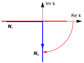
To visualize the situation, we plot the Fourier line of integration along the horizontal axis in blue and (infinite) contour L in the half-plane Im k ≤ 0 (identified in red).
where L is a contour in the lower half k-plane Im k ≤ 0 obtained from the Fourier straight line by continuous deformation.
This yields the solution u(x, t) for positive x.
This formula represents the solution to the given IBVP in the Ehrenpreis form \eqref{Eq3PDE.1}, where only contour L is not specified yet. Our task for the rest is to explain how to choose this contour L and show that the function \eqref{Eq3PDE.15} satisfies all conditions of the given IBVP.
At this point, we can explain the conditions that L must satisfy as we utilize Eq.\eqref{Eq3PDE.15}. It is clear that L must be situated in the lower half plane Im k ≤ 0 because it is one of the requirements of Jordan's lemma, applied to the integral of the form \(
\int_{-\infty}^{\infty} {\text d} k\, e^{-{\bf j}kx} \rho (k) , \)
for x > 0.
Another condition of Jordan's lemma demands the integrand function ρ(k) to decrease uniformly in the area situated between the Fourier line and contour L. The solution formula \eqref{Eq3PDE.15} contains several integrals and contour L should take into account how each integrand decreases and in what area. For example, the integrals
cannot. Indeed,
you cannot utilize the Fourier line of integration (which is the real axis) in the latter integral over variable k because the corresponding integral
\[
\frac{1}{2\pi} \int_{-\infty}^{\infty} {\text d} k\, e^{-{\bf j}kx} \,
e^{-{\bf j} \alpha\,k^3\, t} \int_0^{\infty} {\text d} \eta \, f (\eta ) \left[ \nu\, e^{{\bf j}k\nu \,\eta} + \nu^2 \,e^{{\bf j}k\nu^2 \eta} \right]
\]
diverges due to the exponential terms
These may have positive real parts, which tells us that the corresponding integrals diverge.
Since we realize that in our problem, the mathematics requires a change of the contour of integration in the inverse Fourier transform formula, the next
question to address deals with the conditions that the contour of integration L should satisfy. Out of all the terms in the solution formula \eqref{Eq3PDE.15}, we need to determine the domain in which the integrals in Eq.\eqref{Eq3PDE.16} converge.
More precisely, we choose a path of integration, called the steepest descent, where the integrand decreases fastest. Since the dispersion relation has the highest degree in k than all other terms, it plays a crucial role in the decay property of the integrand. To achieve this, we consider a complex k-plane and identify the areas where the dispersion relation ω(k) = −jk³α has a negative real part.
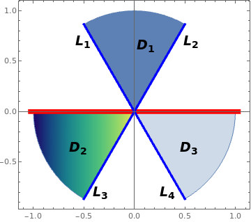
Figure 10: Fourier path of integration (in red) and three subdomains (shaded) where the dispersion relation has a negative real part.
Mathematica code
The Fourier line of integration (-∞, ∞) along the horizontal axes in Figure 10 is shown in red.
There are three wedge-shaped subdomains in the complex k-plane ℂ where the real part of the dispersion relation ω(k) = −jk³α is negative
Hence, the exponential term \( e^{-{\bf j}\,\alpha \,k^3\, T} , \ T > 0,\) tends to zero when |k| → ∞ within D (k∈D). In the white area outside \( \overline{D} , \) the closure of D, this exponential term blows up. On the boundary ∂D, marked by blue lines as well as the horizontal red Fourier line in the picture, the dispersion relation becomes purely imaginary.
To check this conclusion, we select three complex numbers, one
from each of the subdomains D1, D2, and D3, and perform calculations:
\begin{align*}
&{\bf j} \in D_1 \qquad \Longrightarrow \qquad &-{\bf j} \times {\bf j}^3 = -1 ,
\\
&-2 - 3\,{\bf j} \in D_2 \qquad \Longrightarrow \qquad &-{\bf j} \times \left( -2 -3\,{\bf j} \right)^3 = -9-46\,{\bf j} ,
\\
&3 - 2\,{\bf j} \in D_3 \qquad \Longrightarrow \qquad &-{\bf j} \times \left( 3 -2\,{\bf j} \right)^3 = -46 + 9\,{\bf j} .
\end{align*}
Since each complex number has a negative real part, we conclude that the corresponding integrands in Eq.\eqref{Eq3PDE.16} exponentially decay in each of the three regions of D.
Next, we need to determine the domain where Jordan's lemma is valid, so we can transfer the Fourier line of integration into the steepest descent path.
Since the cubic power dominate all lower powers of k, we can stick only with the dispersion relation ω(k).
Hence, we can apply Jordan's lemma in the complex k-plane where the imaginary part
Im k < 0 because x > 0. However, the integrand diverges in white areas. Therefore, we can safely apply Jordan's lemma in D2 ∪ D3.
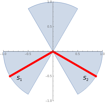
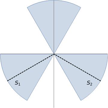
We choose a new path of integration where k3 has an appropriate imaginary part and decreases fastest. So we transfer the negative semi-line (- ∞, 0) of one part of the Fourier integration contour into the line S1 defined by the angle \( \displaystyle e^{{\bf j}\pi + {\bf j}\, \pi /6} = - \frac{\sqrt{3}}{2} - {\bf j}\,\frac{1}{2} \) , and another part (0, ∞) into the line S2 determined by \( \displaystyle e^{- {\bf j}\, \pi /6} = \frac{\sqrt{3}}{2} - {\bf j}\,\frac{1}{2} . \)
Here S = S1∪S2 is the steepest descent path \eqref{Eq3PDE.18}.
Recall that the inverse Fourier transformation is an ill-posed problem. Therefore, its numerical evaluation should be done with care: changing of the order of integration in the integrals in Eq.\eqref{Eq3PDE.15} is not always valid. However, their convergence can be dramatically improved when the Fourier line of integration is transformed within subdomain D2 ∪ D2 (see Figure 10) into a steepest descent path \eqref{Eq3PDE.18} in the complex k-plane ℂ so the resulting integrals will converge rapidly. Then the change of the order of integration can be performed, which will be demonstrated in the following example.
Once the solution formula is obtained and the contour of integration is chosen, we have to verify that all conditions of the given IBVP are satisfied. So its verification is an ingredient of the Fokas method. The crucial part of it is checking initial and boundary conditions because the differential equation is obviously satisfied due to the form of the solution. Note that Jordan's lemma is a part of the verification procedure, but it is not necessarily involved in the solution formula derivation.
The integrals in Eq.\eqref{Eq3PDE.19} can be evaluated either directly or with the aid of Mathematica. Since Mathematica expresses them through special functions; for example,
Now we verify whether our function \eqref{Eq3PDE.15} satisfies the initial and boundary conditions. It needs special attention because the contour of steepest descent S = S1∪S2 works only when t > 0.
Checking the initial condition:
Taking the limit when t → 0 in the first integral containing the initial data in Eq.\eqref{Eq3PDE.15}, we obtain
\[
\frac{1}{2\pi} \int_{L} e^{-{\bf j}kx} \,{\text d} k \int_0^{\infty} e^{{\bf j}k\eta} f(\eta ) \,{\text d} \eta = ℱ_{k\to x}^{-1} \,ℱ_{x\to k} \left[ f(x)\,H(x) \right] = f(x)\,H(x) ,
\]
where H(x) is the Heaviside function and L is an appropriate contour of integration in Im k ≤ 0 (which can be chosen along the Fourier horizontal line, but not necessarily). Therefore, we get
The initial condition will be satisfied if it could be shown that the double integral in the right-hand side of Eq.\eqref{Eq3PDE.20} is zero. The first step in this direction would be determination of a domain where we can deform the steepest descent path S = S1 ∪ S2 without changing the value of the integral. Upon choosing a convenient path, we can evaluate the integrals explicitly.
The double integral above is actually a sum of two integrals: one contains the multiple ν and another one has ν²:
\[
M (x,\eta ) = \frac{\nu}{2\pi} \int_{L} e^{-{\bf j}kx} \, e^{{\bf j}k\nu \,\eta} {\text d} k \qquad \mbox{and} \qquad N (x,\eta ) = \frac{\nu^2}{2\pi} \int_{L} e^{-{\bf j}kx} \, e^{{\bf j}k\nu^2 \,\eta} {\text d} k .
\]
These expressions are obtained upon changing the order of integration in the double integral \eqref{Eq3PDE.20} that converges uniformly along the steepest descent path. Integral M contains an exponential term with the power
\[
{\bf j}k\eta \nu -{\bf j}kx = {\bf j}k\eta \left( -\frac{1}{2} + {\bf j}\,\frac{\sqrt{3}}{2} \right) -{\bf j}kx = - k\eta \,\frac{\sqrt{3}}{2} - {\bf j}\,k \left( \frac{\eta}{2} +x \right) .
\]
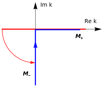
Its real part is negative for k > 0, so we can deform the part S2 into the Fourier half line along the positive real axis. When k < 0, we deform the contour S1 into the path -jL, which is the half-line representing the negative imaginary axis.
The contour of integration with respect to k for the integral
Then
\[
M (x,\eta ) = M_{-} + M_{+} = 0.
\]
Similarly, we consider another integral containing jkην²:
\[
N (x,\eta ) = \frac{\nu^2}{2\pi} \int_{LN} e^{-{\bf j}kx} \, e^{{\bf j}k\nu^2 \,\eta} {\text d} k = N_{-} + N_{+} = \frac{\nu^2}{2\pi} \int_{-\infty}^0 e^{-{\bf j}kx} \, e^{{\bf j}k\nu^2 \,\eta} {\text d} k
+ \frac{\nu^2}{2\pi} \int_{-{\bf j}L} e^{-{\bf j}kx} \, e^{{\bf j}k\nu^2 \,\eta} {\text d} k .
\]
The exponent power for N is
\[
{\bf j}k\eta \nu^2 -{\bf j}kx = {\bf j}k\eta \left( -\frac{1}{2} - {\bf j}\,\frac{\sqrt{3}}{2} \right) -{\bf j}kx = k\eta \,\frac{\sqrt{3}}{2} - {\bf j}k \left( \frac{\eta}{2} + x \right) .
\]
For negative k, its real part is negative and that guarantees its fast convergence of the integral. So we deform the steepest descent line S1 into the negative real part of k. For k > 0, it is positive and we deform S2 into −jL. This guarantees fast decay (exponential) of the integrand.
The contour of integration, which is denoted by LN, with respect to k for the integral
Therefore, the function \eqref{Eq3PDE.15} satisfies the boundary condition u(0, t) = g(t).
It can be shown that the steepest descent path S cannot be deformed into the boundary lines L3 ∪ L4 (see Figure 10) because the corresponding integrals M and N diverge. The same conclusion is valid for integrals along L1 ∪ L2.
▣
Now we calculate the same integral along the blue lines (see Figure 10) of the boundaries of the subdomains Di, i = 1, 2, 3. The boundary of D1 consists of two straight lines:
\[
L_1 = e^{2{\bf j}\pi /3} \,\xi = \left( -\frac{1}{2} + {\bf j}\,\frac{\sqrt{3}}{2} \right) \xi \qquad \mbox{and} \qquad L_2 = e^{{\bf j}\pi /3} \,\xi = \left( \frac{1}{2} + {\bf j}\,\frac{\sqrt{3}}{2} \right) \xi .
\]
Let us work out with these integrals in detail
\begin{align*}
J_1 &= \frac{1}{2\pi} \int_{L_1} {\text d} k\,
e^{-{\bf j} \alpha\,k^3\, t} \left[ e^{{\bf j}k\,\eta} + \nu\, e^{{\bf j}k\nu \,\eta} + \nu^2 \,e^{{\bf j}k\nu^2 \eta} \right]
\\
&= \frac{1}{2\pi} \left( -\frac{1}{2} + {\bf j}\,\frac{\sqrt{3}}{2} \right) \int_{\infty}^0 {\text d} \xi\,
e^{-{\bf j} \alpha\,\xi^3 t} \left[ e^{\left( -\sqrt{3} - {\bf j} \right) \xi\eta /2} + \nu\, e^{\left( \sqrt{3} - {\bf j} \right) \xi\eta /2} + \nu^2 e^{{\bf j} \xi\eta} \right]
\\
&= \frac{-1}{2\pi} \int_0^{\infty} {\text d} \xi \left( A_1 + {\bf j} B_1 \right) e^{-{\bf j} \alpha\,\xi^3 t} ,
\end{align*}
and similarly
\begin{align*}
J_2 &= \frac{1}{2\pi} \int_{L_2} {\text d} k\,
e^{-{\bf j} \alpha\,k^3\, t} \left[ e^{{\bf j}k\,\eta} + \nu\, e^{{\bf j}k\nu \,\eta} + \nu^2 \,e^{{\bf j}k\nu^2 \eta} \right]
\\
&= \frac{1}{2\pi} \left( \frac{1}{2} + {\bf j}\,\frac{\sqrt{3}}{2} \right) \int_0^{\infty} {\text d} \xi\,
e^{{\bf j} \alpha\,\xi^3 t} \left[ e^{\left( - \sqrt{3} + {\bf j} \right) \xi\eta /2} + \nu\,e^{} + \nu^2 e^{} \right]
\\
&= \frac{1}{2\pi} \int_0^{\infty} {\text d} \xi \left( A_2 + {\bf j} B_2 \right) e^{{\bf j} \alpha\,\xi^3 t} ,
\end{align*}
where
Dan Zwillinger
9:13 AM (4 hours ago)
to me
(*) The Fokas picture worked when I checked your web site again.
(*) I modified your code slightly to get sub and super scripts at once (I also increased the font size)
parmplot1 = ParametricPlot[r*{Cos[t], Sin[t]}, {t, Pi/3, 2*Pi/3}, {r, 0, 1}, PlotRange -> All, ImagePadding -> {1, Automatic}];
parmplot2 = ParametricPlot[r*{Cos[t], Sin[t]}, {t, Pi, Pi + Pi/3}, {r, 0, 1}, PlotRange -> All, ImagePadding -> 1];
parmplot3 = ParametricPlot[r*{Cos[t], Sin[t]}, {t, 5*Pi/3, 2*Pi}, {r, 0, 1}, PlotRange -> All];
txt1 = Graphics[Text[Style[ Subsuperscript[D, "1", "-"], FontSize -> 28], {-0.6, -0.4}]];
txt2 = Graphics[Text[Style[ Subsuperscript[D, "2", "-"], FontSize -> 28], { 0.6, -0.4}]];
txt3 = Graphics[Text[Style[ Subsuperscript[D, "", "+"], FontSize -> 28], {-0.15, 0.67}]];
fokasRegions = Show[
ParametricPlot[ r {Cos[t], Sin[t]}, {t, 0, 2 Pi}],
parmplot1, parmplot2, parmplot3, txt1, txt2, txt3,
Ticks -> None]
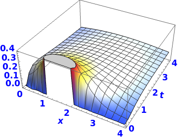
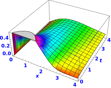
Example:
We consider the problem when the initial function is a piecewise continuous function:
\begin{align*}
&\mbox{PDE:} \qquad &u_t &= -u_{xxx} \qquad\mbox{for } x > 0 \mbox{ and } t > 0, \\
&\mbox{Initial condition:} \qquad &u(x,0) &= f(x) , \qquad x > 0, \\
&\mbox{Boundary condition:} \qquad &u(0,t) &= 0 , \qquad 0 < t < \infty ,
\end{align*}
where
\[
f(x) = H(x-1) - H(x-2) \qquad \mbox{and} \qquad g(t) \equiv 0 ,
\]
with
\[
H(t) = \begin{cases} 1, & \ \mbox{ for } \ t > 0, \\
1/2 , & \ \mbox{ for } \ t =0, \\
0, & \ \mbox{ for } \ t < 0 ,
\end{cases}
\]
being the Heaviside function. Its solution according to Eq.\eqref{Eq3PDE.15} is
Boyd, J.P. and Flyer, N., Compatibility conditions for time-dependent partial differential equations and the rate of convergence of Chebyshev and Fourier spectral methods, Computer Methods in Applied Mechanics and Engineering, 1999, Volume 175, Issues 3–4, Pages 281--309. https://doi.org/10.1016/S0045-7825(98)00358-2
Davis, C.-I. R. and Fornberg, B., A spectrally accurate numerical implementation of the Fokas transform method for Helmholtz-type PDEs, Complex Variables and Elliptic Equations, 2014, Vol. 59, No. 4, pp. 564--577. doi: 10.1080/17476933.2013.766883
Fokas, A.S., A unified transform method for solving linear and certain nonlinear PDEs, Proceedings of the Royal Society. Ser. A: Mathematical, Physical and Engineering Sciences, 453 (1997), 1411-1443.
Fokas, A.S., On the integrability of linear and nonlinear partial differential equations, Journal of Mathematical Physics, 41, 6 (2000), 4188-4237.
Fokas, A.S., A new transform method for evolution PDEs, IMA Journal of Applied Mathematics, 67, 6 (2002), 559-590.
Reference list of publications on Fokas method/unified transform method.
Fokas, A. S. and Gelfand, I. M., Surfaces on Lie groups, on Lie algebras, and their integrability, Communications in Mathematical Physics, 1996, Vol. 177, no. 1, 203--220. https://projecteuclid.org/euclid.cmp/1104286243
Lopatinski Ya. B., A method of reduction of boundary-value problems for systems of differential equations of elliptic type to a system of regular integral equations (in Russian), Ukrainski Mathematical Journal, 1953, Vol. 5, pp. 123--151.
Shapiro Z. Ja.,On general boundary problems for equations of elliptic type (in Russian), Izvestiya Akademii Nauk SSSR, Ser Mat, 1953, Vol. 17, pp. 539--562.
Return to Mathematica page
Return to the main page (APMA0340)
Return to the Part 1 Matrix Algebra
Return to the Part 2 Linear Systems of Ordinary Differential Equations
Return to the Part 3 Non-linear Systems of Ordinary Differential Equations
Return to the Part 4 Numerical Methods
Return to the Part 5 Fourier Series
Return to the Part 6 Partial Differential Equations
Return to the Part 7 Special Functions