Return to computing page for the first course APMA0330
Return to computing page for the second course APMA0340
Return to computing page for the fourth course APMA0360
Return to Mathematica tutorial for the first course APMA0330
Return to Mathematica tutorial for the second course APMA0340
Return to Mathematica tutorial for the fourth course APMA0360
Return to the main page for the first course APMA0330
Return to the main page for the second course APMA0340
Return to the main page for the fourth course APMA0360
Return to Part VII of the course APMA0340
Introduction to Linear Algebra with Mathematica

Preface


The Mathieu equation is an ordinary differential equation with real coefficients. Its standard form with parameters (a, q) is

\begin{equation} \label{EqMathieu.1} w'' + \left( a - 2q\,\cos (2x) \right) w =0 . \end{equation}
It was introduced by the French mathematician Émile Léonard Mathieu (1835--1890) in 1868 in context of the vibrations of an elliptic membrane. Then the equation arises from the separation of variables in the Helmholtz equation
\[ \frac{\partial^2 u}{\partial x^2} + \frac{\partial^2 u}{\partial y^2} + k^2 u = 0 \]
in elliptic coordinates (ξ, η) defined by
\begin{equation} \label{EqMathieu.2} x = a\,\cosh (\xi )\,\cos (\eta ) , \qquad\qquad y = a\,\sinh (\xi )\,\sin (\eta ) , \end{equation}
where (±𝑎, 0) are the cordinates of the ellipse foci, ξ is a nonnegative real number and η ∈ [ 0, 2 π].

On the complex plane, an equivalent relationship is

\[ x + {\bf j} y = a\,\cosh \left( \xi + {\bf j} \eta \right) . \]
These definitions correspond to ellipses and hyperbolae. The trigonometric identity
\[ \frac{x^2}{a^2 \cosh^2 \xi} + \frac{y^2}{a^2 \sinh^2 \xi} = \cos^2 \eta + \sin^2 \eta = 1 \]
shows that curves of constant ξ form ellipses, whereas the hyperbolic trigonometric identity
\[ \frac{x^2}{a^2 \cos^2 \eta} - \frac{y^2}{a^2 \sin^2 \eta} = \cosh^2 \xi - \sinh^2 \xi = 1 . \]
The Laplacian reads
\begin{align*} \nabla^2 \Psi &= \frac{1}{a^2 \left( \sinh^2 \xi + \sin^2 \eta \right)} \left( \frac{\partial^2 \Phi}{\partial \xi^2} + \frac{\partial^2 \Phi}{\partial \eta^2} \right) \\ &= \frac{2}{\cosh 2\xi - \cos 2\eta} \left( \frac{\partial^2 \Phi}{\partial \xi^2} + \frac{\partial^2 \Phi}{\partial \eta^2} \right) . \end{align*}

With[ {\[Alpha] = 1}, ParametricPlot[ { \[Alpha]*Cosh[\[Mu]]*Cos[\[Theta]], \[Alpha]*Sinh[\[Mu]]*Sin[\[Theta]] }, {\[Mu], -2, 2}, {\[Theta], 0, Pi}, PlotRange -> 2*{{-1, 1}, {-1, 1}}, Mesh -> True, PlotStyle -> None ] ]
Add some styling:
With[
{\[Alpha] = 1},
Framed[
ParametricPlot[
{
\[Alpha]*Cosh[\[Mu]]*Cos[\[Theta]],
\[Alpha]*Sinh[\[Mu]]*Sin[\[Theta]]
},
{\[Mu], -2, 2},
{\[Theta], 0, Pi},
PlotRange -> 2*{{-1, 1}, {-1, 1}},
Mesh -> True,
PlotStyle -> None,
MeshFunctions -> {#3 &, #4 &},
MeshStyle -> {
Directive[Opacity[1], Thickness[0.003], Green],
Directive[Opacity[1], Thickness[0.003], Blue]
},
Epilog -> {Red, PointSize -> 0.02,
Point[{{-\[Alpha], 0}, {\[Alpha], 0}}]},
Frame -> False,
Ticks -> {None, Range[0, 10, 0.2]},
GridLines -> Automatic ],
FrameStyle -> Gray, FrameMargins -> 0 ]
]
Elliptic coordinate system

Elliptic coordinate system

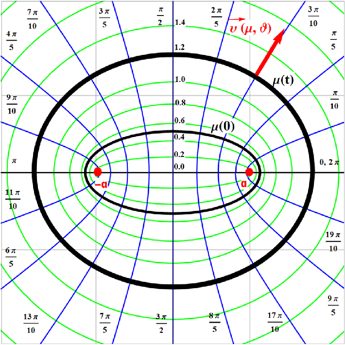
To create an ellipse, fix the value of ξ:

With[ {\[Alpha] = 2, \[Mu] = 2}, ParametricPlot[ {\[Alpha]*Cosh[\[Mu]]*Cos[\[Theta]], \[Alpha]*Sinh[\[Mu]]* Sin[\[Theta]]}, {\[Theta], 0, 2*Pi}, PlotRange -> 20*{{-1, 1}, {-1, 1}} ] ]
Likewise, to create one of the normal curves, fix the value of η.
Use Show to combine two parametric plots:

With[ {\[Alpha] = 1, \[Mu]Fixed = 1}, Framed[ Show[ (* Original plot: *) ParametricPlot[ {\[Alpha]*Cosh[\[Mu]]*Cos[\[Theta]], \[Alpha]*Sinh[\[Mu]]* Sin[\[Theta]]}, {\[Mu], -2, 2}, {\[Theta], 0, Pi}, PlotRange -> 2*{{-1, 1}, {-1, 1}}, Mesh -> True, PlotStyle -> None, MeshFunctions -> {#3 &, #4 &}, MeshStyle -> { Directive[Opacity[1], Thickness[0.003], Green], Directive[Opacity[1], Thickness[0.003], Blue] }, Epilog -> {Red, PointSize -> 0.02, Point[{{-\[Alpha], 0}, {\[Alpha], 0}}]}, Frame -> False, Ticks -> {Automatic, Range[0, 10, 0.2]}, GridLines -> Automatic ] , (* Highlighted ellipse: *) ParametricPlot[ {\[Alpha]*Cosh[\[Mu]Fixed]*Cos[\[Theta]], \[Alpha]* Sinh[\[Mu]Fixed]*Sin[\[Theta]]}, {\[Theta], 0, 2*Pi}, PlotStyle -> Red ] ], FrameStyle -> Gray, FrameMargins -> 0 ] ]

Calculate the radius of an ellipse

The radius of each ellipse is given by the following code:

radius[\[Alpha]_, \[Mu]_, \[Theta]_] := Norm[{\[Alpha]*Cosh[\[Mu]]*Cos[\[Theta]], \[Alpha]*Sinh[\[Mu]]* Sin[\[Theta]]}]; radius[\[Alpha], \[Mu], \[Theta]]
Sqrt[Abs[\[Alpha] Cos[\[Theta]] Cosh[\[Mu]]]^2 + Abs[\[Alpha] Sin[\[Theta]] Sinh[\[Mu]]]^2]

This expression simplifies at the points where the ellipse crosses the axes (that is, when η = 0, η = π/2, η = π or η = (3π)/2):

TableForm[ Join[ {{"Eta", "Radius"}}, Map[{#, radius[\[Alpha], \[Mu], #]} &, {0, Pi/2, Pi, 3*Pi/2}] ] ]

Eta       Radius
0       Abs[\[Alpha] Cosh[\[Mu]]]
π/2       Abs[\[Alpha] Sinh[\[Mu]]]
π       Abs[\[Alpha] Cosh[\[Mu]]
3π/2       Abs[\[Alpha] Sinh[\[Mu]]

radius[1, 1, 0] // N
1.54308

radius[1, 1, Pi/2] // N
1.1752

Experiment with ξ and η

Change the value of ξ:

With[ {\[Alpha] = 2}, Manipulate[ ParametricPlot[ { \[Alpha]*Cosh[\[Mu]]*Cos[\[Theta]], \[Alpha]*Sinh[\[Mu]]*Sin[\[Theta]] }, {\[Theta], 0, 2*Pi}, PlotRange -> 20*{{-1, 1}, {-1, 1}} ], {{\[Mu], 1, "Mu"}, 0, Pi} ] ]

Change the value of θ:

With[ {\[Alpha] = 2}, Manipulate[ ParametricPlot[ { \[Alpha]*Cosh[\[Mu]]*Cos[\[Theta]], \[Alpha]*Sinh[\[Mu]]*Sin[\[Theta]] }, {\[Mu], -100, 100}, PlotRange -> 20*{{-1, 1}, {-1, 1}} ], {{\[Theta], 1, "Theta"}, 0, Pi} ] ]
Solving Helmholtz equation in elliptic coordinates: Rewriting the Helmholtz equation
\[ \nabla^2 u + k^2 u =0 \]
in elliptic coordinates, we get

Mathieu Functions


However, Mathieu's equation and its generalisations are more important than this single application would suggest. This equation is encountered in many different issues in physics, engineering and industry, including the stability of floating ships and railroad trains, the motion of charged particles in electromagnetic Paul traps, the theory of resonant inertial sensors, and many other problem (see expositions by McLachlan and Ruby).

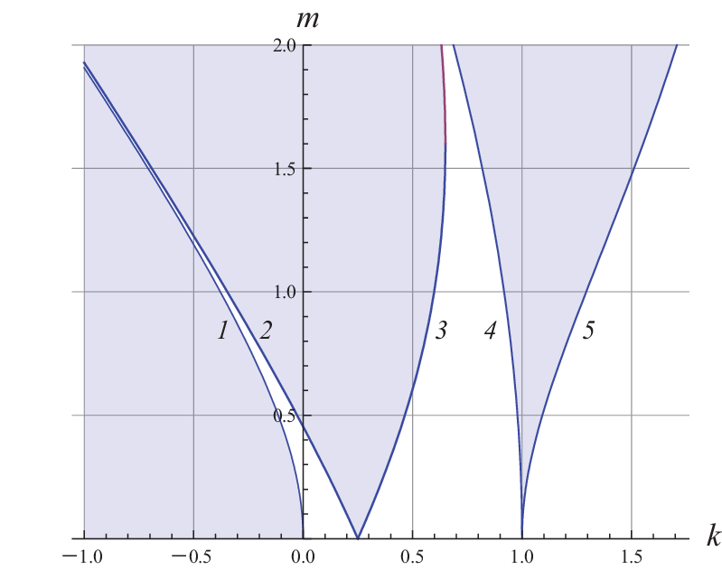
The Mathieu equation has two types of solutions---stable and unstable, depending only on parameters 𝑎 and q and not on the initial conditions.

      Mathieu Stability Chart plots the stable and unstable zones in the plane is known as the Ince--Strutt diagram.
y1[x_] = 2*Sqrt[(x*(x - 1)*(x - 4))/(3*x - 8)];
p1 = Plot[y1[x], {x, -1, 0}, PlotStyle -> Thickness[0.01], AspectRatio -> 1, Filling -> Axis, PlotRange -> {-1, 2}];
y2[x_] = .25*((((9 - 4*x)*(13 - 20*x))^{1/2}) - (9 - 4*x));
p2 = Plot[y2[x], {x, -1, 1/4}, PlotStyle -> Thickness[0.01], AspectRatio -> 1, Filling -> Top, PlotRange -> {-1, 2}];
y3[x_] = (1/4)*((9 - 4*x) - ((9 - 4*x)*(13 - 20*x))^(.5));
p3 = Plot[y3[x], {x, 1/4, 13/20}, PlotStyle -> Thickness[0.01], AspectRatio -> 1, Filling -> Top, PlotRange -> {-1, 2}];
y4[x_] = .25*((9 - 4*x) + ((9 - 4*x)*(13 - 20*x))^(.5));
p4 = Plot[y4[x], {x, 1/4, 13/20}, PlotStyle -> Thickness[0.01], AspectRatio -> 1, Filling -> Top, PlotRange -> {-1, 2}];
y5[x_] = ((2*(x - 1)*(x - 4)*(x - 9))/(x - 5))^(.5);
p5 = Plot[y5[x], {x, 13/20, 1}, PlotStyle -> Thickness[0.01], AspectRatio -> 1, Filling -> Top, PlotRange -> {-1, 2}];
y6[x_] = 2*((x*(x - 1)*(x - 4))/(3*x - 8))^(.5);
p6 = Plot[y6[x], {x, 1, 2}, PlotStyle -> Thickness[0.01], AspectRatio -> 1, PlotRange -> {-1, 2}, Filling -> Top];
Show[p1, p2, p3, p4, p5, p6, PlotRange -> {-1, 2}]
       Fig.1 Ince-Strutt diagram.            Mathematica code.

Fig.1 Ince-Strutt diagram

It is convenient to write Mathieu equation using a slightly different notation from that in Eq. \eqref{EqMathieu.1}, a notation which will be more convenient for our further discussion, namely, as

\begin{equation} \label{EqMathieu.2} \frac{{\text d}^2 u}{{\text d} t^2} + k \left( 1 - m\,\cos t \right) u = 0. \end{equation}
For the great majority of problems associated with the Mathieu equation, the crucial issue is the determination of conditions in which solutions to this equation remain bounded in the course of time, or grow indefinitely. The answer to this question is given by the well-known Ince-Strutt diagram (Figure 1), which shows the transition curves in the parameters plane. These curves divide the plane (k, m) into regions that correspond to unbounded (unstable) solutions (shaded areas in Figure 1) and stable motions.

E.Butikov showed that the transition curves of the Ince-Strutt diagram can be determined by equations:

\begin{align*} m(k) &= 2 \sqrt{\frac{k \left( k-1 \right)\left( k-4 \right)}{3k-8}} \qquad \mbox{for} \quad k < 0; \\ m(k) &= \frac{1}{4} \left( \sqrt{ \left( 9 - 4k \right) \left( 13-20k \right)} - \left( 9 -4k \right) \right) , \qquad \mbox{for} \quad k < \frac{1}{4} ; \\ m(k) &= \frac{1}{4} \left( 9 - 4k \mp \sqrt{\left( 9-4k \right)\left( 13-20k \right)} \right) , \qquad \mbox{for} \quad \frac{1}{4} < k < \frac{13}{20}; \\ m(k) &= \sqrt{\frac{2 \left( k-1 \right)\left( k-4 \right)\left( k-9 \right)}{k-5}} , \qquad \mbox{for} \quad \frac{13}{20} < k < 1 ; \\ m(k) &= 2 \sqrt{\frac{k \left( k-1 \right)\left( k-4 \right)}{3k-8}} , \qquad \mbox{for} \quad k > 1 . \end{align*}
With \( \zeta = \sin^2 z , \) we obtain the algebraic form of Mathieu’s equation
\[ \zeta \left( 1 - \zeta \right) w'' + \frac{1}{2} \left( 1 - 2\zeta \right) w' + \frac{1}{4} \left( 1 - 2q (1-2\zeta ) \right) w =0 . \]
This equation has regular singularities at 0 and 1; it also has an irregular singular point at infinity.
Example 1: The idea of building traps grew out of molecular-beam physics, mass spectrometry, and particle accelerator physics. It was shown that plane electric and magnetic multipole fields are able to focus particles in two dimensions acting on the magnetic or electric dipole moment of the particles. In the electric quadrupole field the potential is quadratic in the Cartesian coordinates. The Laplace equation imposes a two dimensional model
\[ \Phi = \frac{\Phi_0}{2r_0^2} \left( x^2 - z^2 \right) . \]
The equation of motion are
\begin{align*} \ddot{x} + \frac{e}{m r_0^2} \left( U + V \,\cos \omega t \right) x &= 0 , \\ \ddot{z} - \frac{e}{m r_0^2} \left( U + V \,\cos \omega t \right) z &= 0 , \end{align*}
where U is a dc voltage and V is an rf voltage.    ■
Example 2: Ship motion can be described by the following equation
\[ \left( {\bf M} + {\bf A} \right) \ddot{\phi} + D(\ddot{\phi})\,\dot{\phi} + C_{res} (\phi , \eta ) = C{ext} (\eta , \dot{\eta}, \ddot{\eta}) , \]
   ■
Example 3: A simple model for the motion of a conduction electron in a crystal lattice consists of the time-independent Schrödinger equation with a potential that varies periodically in space. This potential describes the effect of the forces due to the ions in the crystal lattice and the other electrons in the crystal on the motion of the electron.

Let us consider the one-dimensional version of this problem. The wavefunction of the electron then satisfies the one-dimensional Schrodinger equation in which the potential V(x) is a periodic function. Suppose that the period is a, so that V(x+a)=V(x). Then, after making the change of variables


\( u(x) = \varphi (x/a) , q(x) = (2ma^2)/h V(x/a), \lambda = 2mE/h^2 , \)

the normalized wavefunction u(x) and energy parameter λ satisfy

\( -u'' + q(x) u = \lambda * u \)

where \( q(x+1) =q(x) . \) We consider this Sturm--Liouville problem on the real line with a general 1-periodic potential q(x), assumed continuous.
A specific example of such an equation is the Mathieu equation:

\( -u'' +2k \,\cos (2x) u = \lambda u , \)

where k is a real paarmeter. Its solutions, called the Mathieu functions, have been studied extensively.

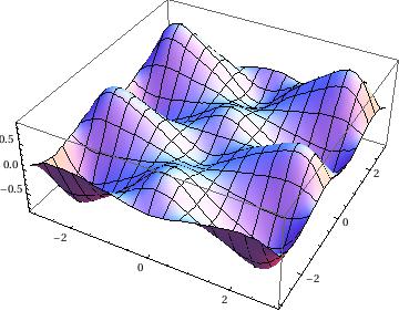
Next we plot Mathieu function:

Plot3D[MathieuC[3,-3/2,x] * MathieuS[5, -3/2,y], {x, -3, 3}, {y, -3, 3}]


  1. Allievi, A. and Soudack, A., Ship stability via the Mathieu equation, International Journal of Control, 1990, Volume 51, Issue 1, pp. 139--167. https://doi.org/10.1080/00207179008934054
  2. Butikov, Eugene I., Analytical expressions for stability regions in the Ince–Strutt diagram of Mathieu eqution, American Journal of Physics, 86, Isuue 4, 257 (2018); https://doi.org/10.1119/1.5021895
  3. Daniel, D.J., Exact solutions of Mathieu’s equation, Progress of Theoretical and Experimental Physics, 2020, Volume 2020, Issue 4, April 2020, 043A01, https://doi.org/10.1093/ptep/ptaa024
  4. Jovanoski, Z. and Robinson, G., Ship Stability and Parametric Rolling, Australasian Journal of Engineering Education, Volume 15, 2009 - Issue 2, pp. 43--50. https://doi.org/10.1080/22054952.2009.11464028
  5. Mathieu, É.L., Memoir on vibrations of an elliptic membrane, 1868; Mémoire sur le mouvement vibratoire d'une membrane de forme elliptique, Journal de Mathématiques Pures et Appliquées 13, 137–203 (1868);
  6. McLachlan, N.W., Theory of Application of Mathieu Functions, Dover, New York, 1964.
  7. Paul, W., Electromagnetic traps for charged and neutral particles, Reviews of Modern Physics, 1990, Vol. 62, No. 3, pp. 531--540. http://dx.doi.org/10.1103/RevModPhys.62.531 )
  8. Rand, R.H., Lecture Notes in Nonlinear Vibrations (new edition). Published on-line by The Internet-First University Press (Cornell's digital repository), 2012.
  9. Ruby, L., Applications of the Mathieu equation, American Journal of Physics, 1995, Volume 64, Issue 1 https://doi.org/10.1119/1.18290


Return to Mathematica page

Return to the main page (APMA0340)
Return to the Part 1 Matrix Algebra
Return to the Part 2 Linear Systems of Ordinary Differential Equations
Return to the Part 3 Non-linear Systems of Ordinary Differential Equations
Return to the Part 4 Numerical Methods
Return to the Part 5 Fourier Series
Return to the Part 6 Partial Differential Equations
Return to the Part 7 Special Functions