Return to computing page for the first course APMA0330
Return to computing page for the second course APMA0340
Return to Mathematica tutorial for the first course APMA0330
Return to Mathematica tutorial for the second course APMA0340
Return to the main page for the first course APMA0330
Return to the main page for the second course APMA0340
Return to Part VII of the course APMA0340
Introduction to Linear Algebra with Mathematica

Preface


Chebyshev polynomials form a special class of orthogonal polynomials especially suited for approximating and polynomial interpolation of other functions. They are widely used in many areas of numerical analysis: uniform approximation, least-squares approximation, numerical solution of ordinary and partial differential equations (the so-called spectral or pseudospectral methods), and so on.

Chebyshev Equations


Pafnuty Chebyshev

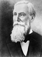
Chebyshev differential equations (actually, there are four of them) were discovered in 1859 by the famous Russian mathematician Pafnuty Lvovich Chebyshev (1821--1894). All these equations are used in definitions of singular Sturm--Liouville problems that ask to find bounded (polynomial) solutions on the interval [−1, 1]. Since these differential equations have two regular singular points at x = ±1, Chebyshev equations have two linearly independent solutions, one of them is unbounded at singular points. It is possible to "explicitly" identify polynomial solutions of these equations that now bear Chebyshev name.

Although Chebyshev's equations do not occur often in physical sciences or engineering, solutions of Chebyshev's equation are of importance in numerical analysis such as approximations of solutions to partial differential equations, smoothing of data, etc. Two singular points x = ±1 divide the real axis ℝ into three intervals, (−∞, −1), (−1, 1), (1, ∞), and Chebyshev's equations can be solved in each of them, we consider these equations only within compact interval [−1, 1].

The Chebyshev polynomials are named after Pafnuty Chebyshev, who invented them in 1859 while solving a practical problem for converting horizontal movement of piston in stream engine into rotational one. Of course, contemporary rail road trains have nothing in common with old steam engines first used in 19 century. His name can be alternatively transliterated as Chebychev, Chebysheff, Chebychov, Chebyshov; or Tchebychev, Tchebycheff (French transcriptions); or Tschebyschev, Tschebyschef, Tschebyscheff, Tschebyschow (German transcriptions). He also used two Russian spellings: Чебышёв and Чебышо́в.

There are four known Chebyshev polynomials, denoted by Tn(x), Un(x), Vn(x), and Wn(x). They all are eigenfunctions of the following singular Sturm--Liouville problems:

\begin{align*} \left( 1 - x^2 \right) y'' - x\, y' + \lambda\,y &=0 , \qquad \lambda = n^2 , \quad y= T_n (x) , \tag{T.1} \\ \left( 1 - x^2 \right) y'' - 3x\, y' + \lambda\,y &=0 , \qquad \lambda = n(n+2) , \quad y = U_n (x) , \tag{U.1} \\ \left( 1 - x^2 \right) y'' - \left( 2x -1 \right) y' + \lambda\,y &=0 , \qquad \lambda = n(n+1) , \quad y = V_n (x) , \tag{V.1} \\ \left( 1 - x^2 \right) y'' - \left( 2x +1 \right) y' + \lambda\,y &=0 , \qquad \lambda = n(n+1) , \quad y = W_n (x) . \tag{W.1} \end{align*}
These problems include the corresponding differential equation and a condition that they have a polynomial solution. The latter can be replaced by the condition:
\[ y(-1) < \infty , \qquad y(1) < \infty . \tag{2} \]

Chebyshev Polynomials of the First Kind


Chebyshev differential equation of the first kind

\[ \left( 1 - x^2 \right) y'' - x\, y' + n^2 y =0 , \qquad n=0,1,2,3,\ldots , \tag{T.3} \]
can be explicitly solved by substitution
\[ x = \cos \theta \qquad \Longrightarrow \qquad \frac{{\text d}x}{{\text d} \theta} = - \sin \theta . \]
Then in new variable, Chebyshev's equation (T.3) becomes
\[ \frac{{\text d}^2 y}{{\text d} \theta^2} + n^2 y = 0 \]
because
\[ y' = \frac{{\text d}y}{{\text d}x} = - \frac{1}{\sin \theta}\, \frac{{\text d}y}{{\text d}\theta} , \qquad y'' = \frac{{\text d}^2 y}{{\text d} x^2} = \frac{1}{\sin \theta} \, \frac{{\text d}}{{\text d}\theta} \left( \frac{1}{\sin \theta}\, \frac{{\text d}y}{{\text d}\theta} \right) . \]
Although the differential equation \( y_{\theta \theta} + n^2 y = 0 \) has two linearly independent solutions y1 = cos(nθ) and y2 = sin(nθ), only former provides a polynomial solution to the Chebyshev equation (T.1). This polynomial solution is known as the Chebyshev polynomial of the first kind, denoted by
\[ T_n (x) = \cos \left( n\,\arccos x \right) , \qquad n = 0,1,2,3,\ldots ; \tag{T.4} \]
and determined by Rodrigues' formula
\[ T_n (x) = \frac{(-1)^n 2^n n!}{(2n)!} \,\sqrt{1-x^2} \,\frac{{\text d}^n}{{\text d}x^n} \left( 1 - x^2 \right)^{n-1/2} , \qquad n=0,1,2,\ldots . \tag{T.5} \]
The name "Rodrigues formula" was introduced by a German mathematician Eduard Heine (1821--1881) in 1878, after Charles Hermite pointed out in 1865 that a French banker, mathematician, and social reformer Rodrigues (1795--1851) was the first to discover it. Chebyshev polynomials can be defined for arbitrary real argument:
\begin{align*} T_n (x) &= \frac{1}{2} \left[ \left( x + \sqrt{x^2 -1} \right)^n + \left( x - \sqrt{x^2 -1} \right)^n \right] \qquad \mbox{for} \quad |x| \ge 1, \\ &= \begin{cases} \cos \left( n\,\mbox{arccos} x \right) , & \quad \mbox{if $|x| \le 1$}, \\ \cosh \left( n\,\mbox{arccosh} x \right) , & \quad \mbox{if $x\ge 1$}, \\ (-1)^n \cosh \left( n\,\mbox{arccosh} (-x) \right) , & \quad \mbox{if $x\le -1$}; \end{cases} \\ &= x^n \sum_{k=0}^{\lfloor n/2 \rfloor} \,\binom{n}{2k} \left( 1- x^{-2} \right)^k . \end{align*}

Another option to define the Chebyshev polynomials directly through explicit formula:

CT[n_, x_] := Module[{k, tmp, tab}, If[n == 0, Return[1]];
If[n == 1, Return[x]];
tmp = (2*x)^n/2;
tab = Table[
tmp = -tmp/4/k*(n - 2*k + 2)*(n - 2*k + 1)/x^2/(n - k), {k, 1, Floor[n/2]}];
(2*x)^n/2 + Apply[Plus, tab]]

Chebyshev Polynomials of the Second Kind


Chebyshev differential equation of the second kind
\[ \left( 1 - x^2 \right) y'' - 3x\, y' + n\left( n+2 \right) y =0 , \qquad n=0,1,2,3,\ldots , \tag{U.3} \]
also can be solved by substitution \( x= \cos t \) or \( x= \cosh t \) depending whether |x| is less than 1 or greater than 1. Chebyshev's polynomials of the second kind satisfy the identity:
\[ U_n \left( \cos \theta \right) = \frac{\sin (n+1)\theta}{\sin \theta} , \qquad \theta \in [0, \pi ], \quad n=0,1,2,\ldots . \tag{U.4} \]
They can be determined by Rodrigues' formula
\[ U_n (x) = \frac{(-1)^n 2^n (n+1)!}{(2n+1)!} \,\frac{1}{\sqrt{1-x^2}} \,\frac{{\text d}^n}{{\text d}x^n} \left( 1 - x^2 \right)^{n+1/2} , \qquad n=0,1,2,\ldots . \tag{U.5} \]
In general, we have
\begin{align*} U_n (x) &= \frac{1}{2\,\sqrt{x^2 -1}} \left[ \left( x + \sqrt{x^2 -1} \right)^{n+1} - \left( x - \sqrt{x^2 -1} \right)^{n+1} \right] = \frac{\sinh \left( (n+1)\,\mbox{arccosh} \,x \right)}{\sinh \left( \mbox{arccosh} \,x \right)} \qquad \mbox{for} \quad |x| \ge 1, \\ &= \frac{\sin \left( (n+1)\,\mbox{arccos} \,x \right)}{\sin \left( \mbox{arccos} \,x \right)} = \frac{\sin \left( (n+1)\,\mbox{arccos} \,x \right)}{\sqrt{1-x^2}} \quad \mbox{for } |x| \le 1; \\ &= x^n \sum_{k=0}^{\lfloor n/2 \rfloor} \,\binom{n+1}{2k+1} \left( 1- x^{-2} \right)^k . \end{align*}


Chebyshev Polynomials of the Third Kind


Chebyshev differential equation of the third kind
\[ \left( 1 - x^2 \right) y'' - \left( 2x -1 \right) y' + n\left( n+1 \right) y =0 , \qquad n=0,1,2,3,\ldots , \tag{V.3} \]
has a polynomial solution
\[ V_{n} (x) = \frac{\cos \left( \frac{2n+1}{2}\,\theta \right)}{\cos \left( \frac{\theta}{2} \right)} = \sum_{k = \lceil n/2 \rceil}^n \binom{k}{n-k} 2^{2k-n-1} (-1)^{n-k} x^{2k-n-1} \left( 2x -2 + \frac{n}{k} \right) , \quad n\ge 2, \qquad x= \cos\theta , \qquad n=0,1,2,\ldots . \tag{V.4} \]
V[n_] = FullSimplify[((x + Sqrt[x^2 - 1])^(n + 1) + (x - Sqrt[x^2 - 1])^(n) )/(Sqrt[x^2 - 1] + x + 1)]
\[ V_{n} (x) = \frac{\left( x + \sqrt{x^2 -1} \right)^{n+1} + \left( x - \sqrt{x^2 -1}\right)^{n}}{x+1+\sqrt{x^2 -1}} , \qquad n=0,1,2,\ldots . \]
They can be determined by Rodrigues' formula
\[ V_n (x) = \frac{(-1)^n 2^n n!}{(2n)!} \,\sqrt{\frac{1-x}{1+x^2}} \,\frac{{\text d}^n}{{\text d}x^n} \left[ \left( 1 - x^2 \right)^{n} \sqrt{\frac{1+x}{1-x}} \right] , \qquad n=0,1,2,\ldots . \tag{V.5} \]


Chebyshev Polynomials of the Fourth Kind


Chebyshev differential equation of the fourth kind
\[ \left( 1 - x^2 \right) y'' - \left( 2x +1 \right) y' + n\left( n+1 \right) y =0 , \qquad n=0,1,2,3,\ldots , \tag{W.3} \]
has a polynomial solution
\[ W_n (x) = \frac{\sin \left( \frac{2n+1}{2}\,\theta \right)}{\sin \left( \frac{\theta}{2} \right)} = \sum_{k = \lceil n/2 \rceil}^n \binom{k}{n-k} 2^{2k-n-1} (-1)^{n-k} x^{2k-n-1} \left( 2x +2 - \frac{n}{k} \right) , \quad n\ge 2, , \qquad x= \cos\theta , \qquad n=0,1,2,\ldots . \tag{W.4} \]
W[n_] = FullSimplify[((x + Sqrt[x^2 - 1])^(n + 1) - (x - Sqrt[x^2 - 1])^(n) )/(Sqrt[x^2 - 1] + x - 1)]
\[ W_{n} (x) = \frac{\left( x + \sqrt{x^2 -1} \right)^{n+1} - \left( x - \sqrt{x^2 -1}\right)^{n}}{x-1+\sqrt{x^2 -1}} , \qquad n=0,1,2,\ldots . \]
They can be determined by Rodrigues' formula
\[ W_n (x) = \frac{(-1)^n 2^n n!}{(2n)!} \,\sqrt{\frac{1+x}{1-x^2}} \,\frac{{\text d}^n}{{\text d}x^n} \left[ \left( 1 - x^2 \right)^{n} \sqrt{\frac{1-x}{1+x}} \right] , \qquad n=0,1,2,\ldots . \tag{W.5} \]
The leading coefficient of polynomial Wn(x) is 2n.


  1. Davis, P., Interpolation and Approximation, ‎ Dover Publications; 2014, ISBN-13 ‏ : ‎ 978-0486624952
  2. Chebyshev, P., L. "Sur le développement des fonctions à une seule variable." Bull. Ph.-Math., Acad. Imp. Sc. St. Pétersbourg 1, 193-200, 1859.
  3. Gasull, A., Li, C., Torregrosa, J., A new Chebyshev family with applications to Abel equations, Journal of Differential Equations, 2012, Volume 252, Issue 2, 15 January 2012, Pages 1635-1641; https://doi.org/10.1016/j.jde.2011.06.010
  4. Mason, J.C. and Handscomb, D.C., Chebyshev Polynomials, (Chapman and Hall/CRC, Boca Raton, 2003).
  5. Rivlin, T.J., Chebyshev Polynomials, Wiley, 1974.
  6. Rivlin, T.J., Chebyshev Polynomials: From Approximation Theory to Algebra and Number Theory, Wiley, 2nd edition, 1990. ISBN-13 ‏ : ‎ 978-0471628965


Return to Mathematica page
Return to the main page (APMA0340)
Return to the Part 1 Matrix Algebra
Return to the Part 2 Linear Systems of Ordinary Differential Equations
Return to the Part 3 Non-linear Systems of Ordinary Differential Equations
Return to the Part 4 Numerical Methods
Return to the Part 5 Fourier Series
Return to the Part 6 Partial Differential Equations
Return to the Part 7 Special Functions