Return to computing page for the first course APMA0330
Return to computing page for the second course APMA0340
Return to Mathematica tutorial for the first course APMA0330
Return to Mathematica tutorial for the second course APMA0340
Return to the main page for the first course APMA0330
Return to the main page for the second course APMA0340
Return to Part VI of the course APMA0340
Introduction to Linear Algebra with Mathematica
Laplace's equation (also called the potential equation or harmonic equation) is a second-order
partial differential equation named after Pierre-Simon
Laplace who, beginning in 1782, studied its properties while investigating the gravitational attraction of arbitrary bodies in space. However, the equation first appeared in 1752 in a paper by
Euler on hydrodynamics. Laplace's equation is often written as:
where \( \Delta = \nabla^2 = \frac{\partial^2}{\partial x_1^2} + \frac{\partial^2}{\partial x_2^2} + \cdots + \frac{\partial^2}{\partial x_n^2} \) is the Laplace operator or Laplacian in n dimensional space. Here Ω is some region in ℝn with smooth boundary.
In two dimensions, the Laplace equation in rectangular coordinates becomes
named after the German physician and physicist Hermann von Helmholtz (1821--1894).
If the region Ω extends to infinity, then it is assumed that a solution to the Laplace's or Helmholtz's equation satisfies additional constraint: it should approach zero at infinity for dimensions larger than 2. In two dimensions, it is sufficient to require soundness of the solution.
where f is a given smooth function, is called the
Poisson's equation. The equation is named after the French mathematician, geometer, and physicist Siméon Denis Poisson (1781--1840).
The Poisson's equation in three dimensional case is
\[
u_{xx} + u_{yy} + u_{zz} = f(x,y,z) ,
\]
where f is a given smooth function.
A particular solution of the Poisson equation \( \Delta u = f \) is given by
gives a particular solution to the Poisson's equation for the Laplacian,
where ωn is the surface area of the unit sphere
\( x_1^2 + x_2^2 + \cdots + x_n^2 =1 . \)
The Laplacian occurs in different situations that describe many physical phenomena, such as electric and gravitational potentials, the diffusion equation for heat and fluid flow, wave propagation, and quantum mechanics. The Laplacian represents the flux density of the gradient flow of a function. For instance, the net rate at which a chemical dissolved in a fluid moves toward or away from some point is proportional to the Laplacian of the chemical concentration at that point. We summarize the standard examples of its applications in the following table.
Application
u
f
Incompressible irrotational flow in two or three dimensions
u = velocity potential, velocity = q = ∇u
Mass source strength/unit volume
Electrostatics
u = electrostatic potential; electric field = E = ∇u
Charge/unit volume
Steady state temperature in a solid
u = temperature
Heat source strength/unit volume
Two dimensional incompressible steady flow
u = stream function = ψ = velocity = q = ψxi - ψyj
-Vorticity
Static deflection of a thin membrane in two dimensions
u = deflection
Pressure
Newtonian gravitation
u = gravitational potential; force of gravity = F = - ∇u
Mass density
Laplace's or Helmholtz equations have infinite many solutions. To take out one of them, we need to impose some conditions that usually follow from physical counterpart.
Since there is no time dependence in the Laplace's equation or Poisson's equation, there is no initial conditions to be satisfied by their solutions. However, there should be certain boundary conditions on the boundary curve or surface \( \partial\Omega \) of the region Ω in which the differential equation is to be solved. Typically, there are known three types of boundary conditions.
where f is a given function, defined on the boundary \( \partial\Omega . \) The first-type boundary condition is named after the German mathematician Peter Gustav Lejeune Dirichlet (1805--1859).
where n denotes the exterior unit normal vector to the boundary \( \partial\Omega . \) The second-type boundary condition is named after the German mathematician Carl (also Karl) Gottfried
Neumann
(1832--1925).
The third type boundary condition is a type of boundary condition that combines two previously defined boundary conditions:
where a and b are nonzero functions or constants.
The third boundary condition is variously designated, but sometimes it is called Robin's boundary condition, which is
mistakenly associated with the French mathematical analyst Victor Gustave Robin (1855--1897) from the Sorbonne in Paris. Actually, Robin never used this boundary condition as it follows from the historical research article by
Karl Gustafson and Takehisa Abe.
The problem of finding a solution of Laplace's equation that takes on given boundary values is known as a Dirichlet problem. However, if the values of the normal derivative are prescribed on the boundary, the problem is said to be a Neumann boundary value problem. Physically, it is plausible to expect that three types of boundary conditions will be sufficient to determine the solution completely. Indeed, it is possible to establish the existence and uniqueness of the solution of Laplace's (and Poisson's) equation under the first and third type boundary conditions, provided that the boundary \( \partial\Omega \) of the domain Ω is smooth (have no corner or edge). However, we avoid explicit statements and their proofs because the material is beyond the scope of the tutorial. Instead, we concentrate our attention on some typical problems that could be solved by means of separation of variables.
Actually, there are known two kinds of boundary value problems: internal or inner when we are after solutions inside the given domain Ω, and external or outer when solutions are to be found outside the given domain, namely in \( {\mathbb R}^n \setminus \Omega . \)
Uniqueness Theorems:
Dirichlet problem. If two functions are harmonic (Δu = 0) in finite domain Ω and coincide on its smooth boundary ∂Ω, they are identical in Ω.
Neumann problem. If two one-valued functions u1 and u2 are harmonic (Δu = 0) in a finite domain Ω and their normal derivatives coincide on its boundary ∂Ω, then u1 and u2 differ by at most a constant in Ω.
Mixed boundary-value problem. If two functions u1 and u2 are harmonic (Δu = 0) in a finite domain Ω and satisfy the same mixed boundary conditions, then u1 and u2 coincide in Ω. ▣
Note that the above uniqueness theorems are valid also for external boundary value problems.
Often, the Dirichlet boundary value problems arise with discontinuous boundary conditions. If we assume that the function u satisfies Laplace's equation inside the domain Ω, contiguously adjoining the boundary values at the points of continuity of the latter, and bounded in neighborhoods of points of discontinuity, then the solution to the first type boundary value problem is unique.
Gauss' Integral Theorem:
If Δu = 0 in a finite domain Ω ⊂ ℝ³ with smooth boundary ∂Ω, then
where dA is the element of surface and n is a unit outward normal to Ω.
▣
Mean-Value Theorem:
Let P(x,y,z) be a fixed point inside a finite domain Ω ⊂ ℝ³ with smooth boundary ∂Ω, and let Δu = 0 in Ω. Let S be a sphere of radius r centered at P with boundary ∂S lying entirely inside Ω. If Δu = 0 in Ω, then
\[
u(P) = \frac{1}{4\pi r^2}\iint_{\partial S} u \, {\text d}A \qquad\mbox{and in $n$ dimensional case} \qquad u (P) = \frac{1}{s_1 r^{n-1}}\int_{S_r} u \left( Q \right) {\text d}S_Q ,
\]
where Sr is the sphere of radius r centered at P and s1 is the area of the unit sphere.
For two dimensional case (on the plane), we have for a harmonic function (\( \phi_{xx} + \phi_{yy} = 0 \) )
Thus, the value of a harmonic function at any point P is the average of the values it takes on any sphere surrounding that point. ▣
The Principle of Maximum Value:
If the function u(P), defined and continuous in the closed region Ω+∂Ω, satisfies Laplace's equation ∇²u = 0 inside Ω, then maximum and minimum values of the function u(P) are attained on the smooth surface ∂Ω.
Dirichlet’s Principle:
Any classical solution u of the Dirichlet problem for Laplace's equation
\[
\Delta u = 0, \qquad \left. u \right\vert_{\partial\Omega} = f ,
\]
where Ω is a bounded domain in ℝn and f is a given function on the smooth boundary ∂Ω of Ω, minimizes the Dirichlet integral
among all smooth functions taking f on the boundary ∂Ω.
It will be shown in next sections that boundary value problems can be solved without much difficulty for simple two-dimensional regions, such as rectangle, half-plane, circle, and so on, the problem is much more difficult for general domains. There are, of course, methods for approximating and solving boundary value problems such as the method of Balayage (see Tsuji's book), the Perron method, finite-difference methods, finite element method, Monte Carlo method, Galerkin method, and boundary element method to name some, but nevertheless the problem is difficult.
An important technique to solve boundary value problems is integral transformation. We will demonstrate later its applications in some relatively simple domain. For example, the Fourier integrals can be used to determine functions of Laplace's or Helmholtz operators in infinite space ℝn.
The Laplace operator Δ in the space ℝn has only negative eigenvalues, so its negation will be a positive one. We can define its square root (using Fourier transformation) as
where x ∈ ℝn and Cn is a constant.
The real and imaginary part of any holomorphic function yield harmonic functions on ℝ² (these are said to be a pair of harmonic conjugate functions). the Laplace operator on the plane can be decomposed as \( \displaystyle \nabla^2 = \left( \frac{\partial}{\partial x} + {\bf j}\,\frac{\partial}{\partial y} \right) \left( \frac{\partial}{\partial x} - {\bf j}\,\frac{\partial}{\partial y} \right) \) where j is the unit vector in positive vertical direction on the complex plane ℂ, so j² = -1. Therefore, the solution of Laplace's equation in two dimensional domains is intimately related to the theory of analytic functions of a complex variable. This is immediately seen observing that, writing z = x + jy, the complex function g(z) = ux − juy is holomorphic in Ω because it satisfies the Cauchy–Riemann equations. Hence, g has locally a primitive f, and u is the real part of f up to a constant, as ux is the real part of f′ = g. In fact, this topic occupies a significant portion of texts on complex variables, and we are not after it.
Finally, we present two important methods to solve boundary value problems in arbitrary domain. We start with Green's function method, and then go to the reduction to integral equations---the technique used in finite element method.
Although Green's function method could be applied to arbitrary boundary value problem for an elliptic operator
we will mostly demonstrate it for Laplace's equation when
\( L[u] = \nabla^2 u . \) As usual, n denotes a unit outward vector to the boundary ∂Ω of the region Ω.
The Green function method in two and three dimensions is based on the formulas:
respectively. Here rPQ is the distance between points P(x,y,z) and Q(ξ,η,ζ) from ℝ³, and
\( \delta (P,Q) = \delta(x,\xi )\,\delta(y,\eta )\,\delta(z,\zeta ) \)
is the delta function of Dirac. For two dimensional case, points
P(x,y) and Q(ξ,η) depend on two variables.
The Green function for the Poisson equation subject to the boundary conditions
\[
L \left[ u \right] = f \left( P\right) , \qquad \left( a(P)\,u(P) + b(P)\,\frac{\partial u}{\partial {\bf n}} \right)_{P\in\partial\Omega} = 0,
\]
where L is an elliptic operator (of which we consider only either the Laplacian (L = Δ) or Helmholtz operator Δ + k²), is
the function G(P.Q) of two variables/points that is the solution to the specific nonhomogeneous equation and homogeneous boundary conditions:
Once Green's function is obtained, the solution of the corresponding boundary value problem \( \mbox{div}\left( k\,\nabla \,u \right) - q\,u = f , \quad \left( a(P)\,u(P) + b(P)\,\frac{\partial u}{\partial {\bf n}} \right)_{P\in\partial\Omega} = \varphi \) can be expressed explicitly:
for two dimensional case. In the above equations, v(P,Q) is a harmonic functions satisfying the appropriate boundary conditions to compensate the influence of the singular term:
for two dimensional case. The corresponding first kind and third kind boundary value problems for function v have unique solutions. The formulas and statements are valid for outer boundary value problems as well.
Note: Green's function for the Neumann problem cannot be expressed through the above formula
\( G(P,Q) = \frac{-1}{4\pi\,r_{PQ}} + v \) because such function v does not exist because v must be a solution of second kind boundary value problem
Such function φ does not exist since necessary condition \( \int_{\partial\Omega} \varphi \,{\text d}S =0 \) fails.
In this case, Green's functions is defined upon solving the Neumann problem:
Since Green's function is harmonic everywhere except at one point, and because it vanishes at infinity, it has the physical interpretation of being the potential of the electrostatic field due to a point charge. This physical interpretation is of use in constructing Green's functions for some simple domains. Here we demonstrate the method of reflection for finding Green's function for half plane in the following example.
Example:
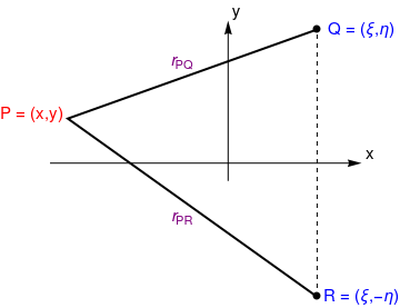
Let us consider first two dimensional case, namely upper half-plane. Green's functions for such region may be interpreted as the deflection of a membrane (which is clamped all along the x-axis) as measured at a point P = (x,y) due to a unit concentrated force at Q = (ξ,η). It is clear from symmetry that the zero boundary condition on y = 0 can be achieved by adding an image force of unit negative strength at point R = (ξ,-η). Thus, we have
It may be interpreted as the velocity potential due to a two-dimensional unit source at Q and an image source of equal strength at R. Now
\( \partial G/\partial{\bf n} = - \partial G/\partial y , \) and it is clear that on y = 0 the normal components of velocity due to the two sources are exactly opposite and cancel out. Note that since the region is infinite, integral over the boundary \( \int_{-\infty}^{\infty} G(P,Q)\,{\text d}x \) does not exist and we have normalized G by requiring its minimum value on the boundary y = 0 to occur at P = (ξ,0).
Now we go to the three dimensional case.
Consider the Dirichlet problem in half space:
\[
\nabla^2 u =0 , \quad -\infty < x < \infty , \quad -\infty < y < \infty , \quad 0 < z < \infty , \qquad u(x,y,0) = f(x,y) .
\]
The solution of this boundary value problem is given by Poisson's integral:
Example:
Let us consider a unit sphere and two points in spherical coordinates P = (r,θ,φ) and Q = (ρϑ,ψ). Then we choose point R = (1/ρ,ϑ,ψ) outside the sphere symmetrical to Q. If we denote the angle POQ by γ, the distance PQ by rPQ and the distance PR by rPR, we have
It is possible to show by direct substitution that if u = f(r,θ,φ) is harmonic inside the sphere of radius R, then v = (R/r)f(R/r,θ,φ) is harmonic outside, and v → 0 as r → ∞.
This is a very interesting formula. It expresses the value of a harmonic function u at any point P inside a domain Ω with smooth boundary in terms of the values of u and
\( \partial u/\partial{\bf n} \) on ∂Ω. However, we know that knowledge of the boundary values of u along as well as its normal derivative is sufficient to determine u in the interior. Therefore, we need a way of eliminating either u or its normal derivative \( \partial u/\partial{\bf n} \) from the above formula. This is the idea for reducing a boundary value problem to an integral equation.
We work with Neumann and Dirichlet boundary value problems in two dimensions:
In the above problems, we assume that u, f, and g are suitably differentiable, and the boundary ∂Ω is smooth.
The mathematical tool required to recast boundary value problems as integral equations is the boundary or surface potential. Although there are different types of boundary potentials, we mostly will deal either with the single-layer boundary potential
The importance of these boundary potentials lies in the fact that first, they both satisfy Laplace's equation ∇² = 0 for any density σ(s) and μ;(s) in such a way that S(x,y) also satisfies the Neumann boundary conditions, and D(x,y) satisfies the Dirichlet boundary conditions. Namely, the following theorems are valid.
Single-layer boundary potential:
Let ∂Ω be a smooth curve containing a region Ω and σ(s) be a single-layer density distribution along ∂Ω. Under these conditions the following properties hold for the single-layer potential S(x,y).
S(x,y) satisfies Laplace's equation ∇²S = 0 inside and outside the boundary ∂Ω.
The single-layer potential S(x,y) is continuous across the boundary ∂Ω.
The outward normal derivative of S(x,y) has a jump discontinuity of 2πσ(ξ,η) across ∂Ω at the point (ξ,η) ∈ ∂Ω.
holds for points (x,y) approaching boundary points (ξ,η) from inside ∂Ω. Correspondingly, when points (x,y) approaching boundary points (ξ,η) from outside ∂Ω, we have
Here index i indicates approaching point at the boundary from inside, while inswz e indicatesd approacing boundary point from outside. Subscript 0 servs for the point at the boundary.
Double-layer boundary potential:
Let ∂Ω be a smooth curve containing a region Ω and μ(s) be a double-layer density distribution along ∂Ω. Under these conditions the following properties hold for the double-layer potential D(x,y).
D(x,y) satisfies Laplace's equation ∇²D = 0 inside and outside the boundary ∂Ω.
The double-layer potential D(x,y) is continuous across the boundary ∂Ω.
The outward normal derivative of D(x,y) is continuous across the boundary ∂Ω.
holds for points (x,y) approaching boundary points (ξ,η) from inside ∂Ω. Correspondingly, when points (x,y) approaching boundary points (ξ,η) from outside ∂Ω, we have
where Di(x,y,z) is the limiting value of the potential of double layer approaching the point P from inside, and De(x,y,z) is the limiting value of the potential of double layer approaching the point P from outside.
The potentials of a sinle and double layer at points of the surface ∂Ω are improper integrals. These integrals converge for a special class of C¹ surfaces called Lyapunov surfaces.
A surface is called a Lyapunov surface, if the following conditions are fulfilled.
At every point of surface ∂Ω there exists a unique normal and tangent surface.
There exists a number d > 0 such that straight lines, parallel to the normal at some point P of the surface ∂Ω intersect a part SP of the surface ∂Ω lying inside a sphere of raius ,i.d,/i. with center P, not more than once. These parts of the surface SP are called the Lyapunov Neighbourhoods.
The angle γ(P,Q) between normal vectors at pomits P and Q satisfies the following inequality
\[
\gamma (P,Q) < A\,r^{\delta} ,
\]
where r is the distance between the points P and Q, A is some positive constant, and 0 < δ ≤ 1.
Example:
Assuming that the density is constant μ(&zi;,η) ≡ 1, then the double layer potential will be
So it experiebces a jump of discontinuity of 2π across ∂Ω.
■
We are now in a position to convert the Neumann and Dirichlet problems to integral equations of Fredholm type. So consider the Dirichlet boundary value problem
Since D(x,y) automatically satisfies Laplace's equation in Ω for any dipole density μ(s), we seek μ(s) so that D(x,y) also satisfies the boundary condition D = f. To do this, recall that D(x,y) has a jump discontinuity across the boundary ∂Ω.
Since we require the solution of the Dirichlet problem to be continuous out to the boundary, we can replace the boundary condition D = f by
where φ is the angle between the normal at the fixed point P(ξ,η) and the line PQ connecting P with varing point Q of integration. The above equation is a Fredholm integral equation of the second kind.
Similarly, we can solve a Neumann problem using a single layer potential
S(x,y). Then using jump discontiuity property of its normal derivative, we arrive at the integral equation
Seeley, R.T., Complex powers of an elliptic operator,
American Mathematical Society, 1967, 20 pages.
Seeley, R.T., The resolvent of an elliptic boundary problem, American Journal of Mathematics, 1969, Vol. 91, No 4, pp. 889--920.
Tsuji, M., Potential theory in mordern function theory, Chelsea, reprint, 1975.
A. D. Wentzell (Ventcel’), On boundary conditions for multidimen-sional diffusion processes, Teoriya Veroiatnostei i ee Primeneniya, translation from Russian in Theory of Probability & Applications, 1959, Vol. 4, Issue 2, pp. 164–177.
Yu, C.L., Reflection principle for solving of higher order elliptic equations with analytic coefficients, SIAM Journal on Applied Mathematics, 1971, Vol. 20, No. 3, pp.358--363.
Return to Mathematica page
Return to the main page (APMA0340)
Return to the Part 1 Matrix Algebra
Return to the Part 2 Linear Systems of Ordinary Differential Equations
Return to the Part 3 Non-linear Systems of Ordinary Differential Equations
Return to the Part 4 Numerical Methods
Return to the Part 5 Fourier Series
Return to the Part 6 Partial Differential Equations
Return to the Part 7 Special Functions
 (born 1937) from Moscow University.