Return to computing page for the first course APMA0330computing page for the second course APMA0340Mathematica tutorial for the first course APMA0330Mathematica tutorial for the second course APMA0340main page for the first course APMA0330main page for the second course APMA0340Part V of the course APMA0340 Linear Algebra with Mathematica
Chebyshev polynomials are usually used for either approximation of continuous functions or function expansion. For the case of functions that are solutions of linear ordinary differential equations with polynomial coefficients (a typical case for special functions), the problem of computing Chebyshev series is efficiently solved by means of Clenshaw’s method.
This section presents some properties of the most remarkable and useful in numerical computations Chebyshev polynomials of first kind \( T_n (x) \) and second kind \( U_n (x) .\) Both Chebyshev polynomials are eigenfunctions of the corresponding singular Sturm--Liouville problems . Other two Chebyshev polynomials of the third kind and the fourth kind are not so popular in applications.
The Chebyshev polynomials of first kind
\( T_n (x) = \cos \left( n\,\mbox{arccos} x \right) \) are solutions of the differential equation
\[
\left( 1- x^2 \right) y'' -x\,y' + n^2 y =0 ,
\]
\( \displaystyle U_n (x) = \frac{\sin \left[ (n+1)\,\arccos x \right]}{\sqrt{1 - x^2}} \) are solutions of the differential equation
\[
\left( 1- x^2 \right) y'' -3x\,y' + n\left( n+2 \right) y =0 ,
\]
\( \displaystyle V_{n} (x) = \frac{\cos \left( \frac{2n+1}{2}\,\theta \right)}{\cos \left( \frac{\theta}{2} \right)} , \) x = cos(θ), are solutions of the differential equation
\[
\left( 1- x^2 \right) y'' - \left( 2x -1 \right) y' + n\left( n+1 \right) y =0 ,
\]
\( \displaystyle W_n (x) = \frac{\sin \left( \frac{2n+1}{2}\,\theta \right)}{\sin \left( \frac{\theta}{2} \right)} , \qquad x= \cos\theta , \) are solutions of the differential equation
\[
\left( 1- x^2 \right) y'' - \left( 2x +1 \right) y' + n\left( n+1 \right) y =0 ,
\]
Chebyshev polynomials form orthogonal sets in weighed vector space 𝔏²[−1, 1] with respect to various
weight functions as in the following inner products:
\begin{align*}
\langle T_n (x), T_m (x) \rangle = \int_{-1}^1 \left( 1 - x^2 \right)^{-1/2} T_n (x) T_m (x) \,{\text d}x &=
\frac{\pi}{{\cal E}_n} \, \delta_{n,m} ,
\\
\langle U_n (x), U_m (x) \rangle = \int_{-1}^1 \left( 1 - x^2 \right)^{1/2} U_n (x) U_m (x) \,{\text d}x &=
\frac{\pi}{2} \, \delta_{n,m} ,
\\
\langle V_n (x), V_m (x) \rangle = \int_{-1}^1 \left( \frac{1+x}{1-x} \right)^{1/2} V_n (x) V_m (x) \,{\text d}x
&= \pi \, \delta_{n,m} ,
\\
\langle W_n (x), W_m (x) \rangle = \int_{-1}^1 \left( \frac{1-x}{1+x} \right)^{1/2} W_n (x) W_m (x) \,{\text d}x
&= \pi \, \delta_{n,m} ,
\end{align*}
where
\[
\delta_{n,m} = \begin{cases} 0, & \ \mbox{if } n \ne m ,
\\
1 , & \ \mbox{if } n = m ; \end{cases} \qquad\quad
{\cal E}_n = \begin{cases} 1 , & \ \mbox{if } n =0, \\
2, & \ \mbox{if } n \ge 1. \end{cases}
\]
and they are orthogonal on the interval [-1, 1] with weight function \( \rho (x) = \left( 1- x^2 \right)^{-1/2} : \)
\[
\int_{-1}^1 \frac{T_m (x)\, T_n (x)}{\sqrt{1-x^2}} \,{\text d} x = \begin{cases}
\pi , & \quad \mbox{if $n=m=0$}, \\
\pi /2 , & \quad \mbox{if $n=m\ne 0$}, \\
0 , & \quad \mbox{if $n\ne m$}. \end{cases}
\]
The Chebyshev polynomials of the second kind
\( U_n (x) \)
are solutions of the differential equation
\[
\left( 1- x^2 \right) y'' -3x\,y' + n(n+2)\, y =0 ,
\]
and they are orthogonal on the interval [-1, 1] with weight function
\( \rho (x) = \left( 1- x^2 \right)^{1/2} : \)
\[
\int_{-1}^1 U_m (x)\, U_n (x)\, \sqrt{1-x^2} \,{\text d} x = \begin{cases}
\pi /2 , & \quad \mbox{if $n=m$}, \\
0 , & \quad \mbox{if $n\ne m$}. \end{cases}
\]
Chebyshev polynomials form a special class of polynomials especially
suited for approximating other functions. They are widely used in many areas
of numerical analysis: uniform approximation, least-squares approximation,
numerical solution of ordinary and partial differential equations (the
so-called spectral or pseudospectral methods), and so on. In the appropriate
Sobolev space , the set of Chebyshev polynomials form an orthonormal basis, so that a function in the same space can, on −1 ≤ x ≤ 1 be expressed via the expansion
\[
f(x) = \frac{a_0}{2} + \sum_{k\ge 1} a_k T_k (x) = \sum_{k\ge 0} b_k U_k (x) =
\sum_{k\ge 0} c_k V_k (x) = \sum_{k\ge 0} d_k W_k (x) .
\]
The Chebyshev polynomials (of any kind) form an orthogonal basis that (among other things) implies that the coefficients can be determined easily through the application of an inner product. This sum is called a
Chebyshev series or a Chebyshev expansion. All of the theorems, identities, etc. that apply to Fourier series have a Chebyshev counterpart.
Arbitrary continuous function can be approximated by Chebyshev
interpolation and Chebyshev series that converges pointwise. If f(x) is continuous in the interval [−1,1] apart from a finite number of step discontinuities in the interior, then its Chebyshev series expansion converges to f wherever f is continuous, and to the average of the left and right limiting values at each discontinuity. To obtain uniform convergence of the Chebyshev series, continuous function f should have bounded variation, similar to Fourier series (Dirichlet or Dini--Lipschitz condition ). If a function is no more than barely continuous, then we can derive uniformly convergent approximations from its Chebyshev expansion by averaging out the partial sums, and thus forming ‘Cesàro sums ’ of the Chebyshev series.
For the case of solutions of linear ordinary differential equations with
polynomial coefficients (a typical case for special functions), the problem of computing
Chebyshev series is efficiently solved by means of Clenshaw’s method .
If function
f (
x ) is defined over closed interval {−1, 1], is absolutely integrable with the weight
\( w (x) = \left( 1- x^2 \right)^{-1/2} , \) then the function can be expanded into Fourier--Chebyshev
\begin{equation} \label{EqCheb1.1}
\frac{f(x+0) + f(x-0)}{2} = \lim_{\varepsilon \downarrow 0} \frac{f(x+ \varepsilon ) + f(x- \varepsilon )}{2} =
\frac{a_0}{2} + \sum_{k\ge 1} \,a_k\, T_{k} (x ) ,
\end{equation}
where
\begin{equation} \label{EqCheb1.2}
a_k = \frac{2}{\pi}\,\int_{-1}^1 \,\frac{f(x)\, T_{k} (x )}{\sqrt{1-x^2}}\, {\text d} x = \frac{2}{\pi}\,\int_{0}^{\pi} \, f\left( \cos \,\theta \right) \cos \left( k\,\theta \right) {\text d} \theta , \qquad k=0,1,2,\ldots .
\end{equation}
Since expansion \eqref{EqCheb1.1} resembles classical Fourier series expansion, we expect to see the Gibbs phenomenon at the points of discontinuity. It is not a surprise that the amounts of overshoot and undershoot at discontinuities are exactly the same as for Fourier series.
Formula \eqref{EqCheb1.2} shows that the Chebyshev expansion \eqref{EqCheb1.1} is actually cosine Fourier expansion of the even function
\( f( \cos \theta ) \) over interval [0, π]. Therefore, all cosine Fourier expansions that were found previously can be automatically applied to the series expansions over Chebyshev polynomials of the first kind. Therefore, the conditions of pointwise convergence of Chebyshev series follow from similar results about Fourier series. In particular, we get
Parseval’s identity :
\[
\frac{a_0^2}{2} + \sum_{n\ge 1} a_n^2 = \frac{2}{\pi}\, \| f \|^2 = \frac{2}{\pi}\, \int_{-1}^1 \left( 1 - x^2 \right)^{-1/2} \left\vert f (x) \right\vert^2 \,{\text d}x .
\]
For example, we found previously in section VIII that
\[
\frac{1}{2} - \frac{\pi}{4}\,|\theta | = \sum_{n\ge 1} \frac{1}{(2n-1)^2} \,\cos (2n-1) \theta , \qquad 0 < \theta < \pi .
\]
We claim that
\[
\frac{1}{2} - \frac{\pi}{4}\,|\arccos x| = \sum_{n\ge 1} \frac{1}{(2n-1)^2} \,T_{2n-1} (x) , \qquad -1 < x < 1 .
\]
Theorem 1:
When a function
f has
m +1 continuous derivatives on [−1,1] and vanishes at endpoints, where
m is a positive integer, then
\( \left\vert f(x) - S_n (x) \right\vert = O\left( n^{-m} \right) \) as
n → ∞ , where
\[
S_n (x) = \frac{a_0}{2} + \sum_{k= 1}^n a_k T_k (x)
\]
is the partial Chebyshev sum.
We can interpolate arbitrary polynomial p n(x ) of degree n :
\[
p_n (x) = \,\sum_{k=0}^{n} \,^{\prime} \, a_{k} \, T_{k} (x) = \frac{a_0}{2} + \sum_{k= 1}^n \,a_k\, T_{k} (x ) ,
\]
where the prime indicates that the term for
k = 0 is to be halved and
\[
a_{k} = \frac{2}{n+1} \,\sum_{j=0}^n \,p(x_j )\, T_{k} (x_j ) , \qquad x_j = \cos \left( \frac{2j+1}{2n+2}\, \pi \right) .
\]
Example 1A: power function expressing through Chebyshev polynomials
Example 1A: x n can be expressed in terms of Chebyshev polynomials as follows:
\[
x^n = 2^{1-n} \,\sum_{k=0}^{\lfloor n/2 \rfloor} \,^{\prime} \, \binom{n}{k} \, T_{n-2k} (x) = T_n (x) + 2^{1-n} \,\sum_{k=1}^{\lfloor n/2 \rfloor} \, \binom{n}{k} \, T_{n-2k} (x) , \qquad n=1,2,\ldots ;
\]
where
\( \binom{n}{k} = \frac{n!}{k! \left( n-k \right) !} \) is the
binomial coefficient and
\( \lfloor \,\cdot \,\rfloor \) is the
floor function .
As usual,
the prime in the sum sign indicates that the term for
k = 0 is to be halved. Similarly,
\[
x^n = 2^{-n} \left[ U_n (x) + \left( n-1\right) U_{n-2} (x) + \cdots \right] , \qquad n=1,2,\ldots .
\]
■
Example 2A: cubic function expressing through Chebyshev polynomials
Example 2A: \( f(x) = 4\,x^3 -1 . \) Since it is a polynomial of degree n = 3 , we can use the corresponding formula to determine the coefficients in Chebyshev series:
\[
c_0 = \frac{2}{4} \,\sum_{j=0}^3 \,f\left( \cos \frac{2j+1}{8}\,\pi \right) = \frac{2}{\pi}\,\int_{0}^{\pi} \, f\left( \cos \,\theta \right) {\text d} \theta = -2,
\]
\[
c_1 = \frac{2}{4} \,\sum_{j=0}^3 \,f\left( \cos \frac{2j+1}{8}\,\pi \right) T_1 \left( \cos \frac{2j+1}{8}\,\pi \right) = \frac{2}{\pi}\,\int_{0}^{\pi} \, f\left( \cos \,\theta \right) \cos \theta \, {\text d} \theta = 3,
\]
\[
c_2 = \frac{2}{4} \,\sum_{j=0}^3 \,f\left( \cos \frac{2j+1}{8}\,\pi \right) T_2 \left( \cos \frac{2j+1}{8}\,\pi \right) = \frac{2}{\pi}\,\int_{0}^{\pi} \, f\left( \cos \,\theta \right) \cos 2\theta \, {\text d} \theta = 0,
\]
\[
c_3 = \frac{2}{4} \,\sum_{j=0}^3 \,f\left( \cos \frac{2j+1}{8}\,\pi \right) T_3 \left( \cos \frac{2j+1}{8}\,\pi \right) = \frac{2}{\pi}\,\int_{0}^{\pi} \, f\left( \cos \,\theta \right) \cos 3\theta \, {\text d} \theta = 1.
\]
Therefore, we get the Chebyshev expansion of the given function:
\[
4x^3 -1 = -1 + 3\, T_1 (x) + T_3 (x) = -1 +3x + \left( 4\,x^3 -3x \right) ,
\]
which is an exact equation. We do similar job with Chebyshev polynomials of the second kind:
\[
4\,x^3 -1 = b_0 \,U_0 + b_1 \,U_1 (x) + b_2 \, U_2 (x) + b_3 \, U_3 (x) = b_0 + b_1 \,2x + b_2 \left( 4x^2 -1 \right) + b_3 \left( 8x^3 -4x \right) ,
\]
where
\begin{align*}
b_0 &= \frac{2}{\pi} \,\int_{-1}^1 \left( 4x^3 -1 \right) \sqrt{1-x^2} \,{\text d} x =
\frac{2}{\pi} \,\int_{0}^{\pi} \left( 4\cos^3 \theta -1 \right) \sin^2 \theta \, {\text d} \theta = -1,
\\
b_1 &= \frac{2}{\pi} \,\int_{-1}^1 \left( 4x^3 -1 \right) \sqrt{1-x^2} \,2x\, {\text d} x =
\frac{2}{\pi} \,\int_{0}^{\pi} \left( 4\cos^3 \theta -1 \right) \sin \theta \,\sin 2\theta {\text d} \theta = 1,
\\
b_2 &= \frac{2}{\pi} \,\int_{-1}^1 \left( 4x^3 -1 \right) \sqrt{1-x^2} \,2x\, {\text d} x =
\frac{2}{\pi} \,\int_{0}^{\pi} \left( 4\cos^3 \theta -1 \right) \sin \theta \,\sin 3\theta {\text d} \theta = 0,
\\
b_3 &= \frac{2}{\pi} \,\int_{-1}^1 \left( 4x^3 -1 \right) \sqrt{1-x^2} \,2x\, {\text d} x =
\frac{2}{\pi} \,\int_{0}^{\pi} \left( 4\cos^3 \theta -1 \right) \sin \theta \,\sin 4\theta {\text d} \theta = \frac{1}{2} .
\end{align*}
Therefore,
\[
4\,x^3 -1 = -U_0 + U_1 (x) + \frac{1}{2} \, U_3 (x) = -1 + 2x + \frac{1}{4} \left( 8x^3 -4x \right) ,
\]
which is the identity.
■
Example 3A: exponential function expressing through Chebyshev polynomials
Example 3A:
\[
e^{a\,\cos\theta} = I_0 (a) + 2 \sum_{n\ge 1} I_n (a)\, \cos n\theta ,
\]
where
I n (𝑎) is the Bessel function of imaginary argument. From this equality follows
\[
e^{a\,x} = I_0 (a) + 2 \sum_{n\ge 1} I_n (a)\, T_n (x) , \qquad x \in [-1, 1] .
\]
In particular, when (𝑎 = 1, we have
\[
e^{x} = I_0 (1) + 2 \sum_{n\ge 1} I_n (1)\, T_n (x) , \qquad x \in [-1, 1] .
\]
Using pure imaginary (𝑎, we obtain
\begin{align*}
\cos ax &= I_0 (a) + 2 \sum_{k\ge 1} (-1)^k J_{2k} (a)\, T_{2k} (x) ,
\\
\sin ax &= 2 \sum_{k\ge 0} (-1)^k J_{2k+1} (a)\, T_{2k+1} (x) .
\end{align*}
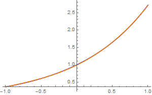
Consider an exponential function \( f(x) = e^x . \)
Its third order Chebyshev approximation is
\[
e^x \approx \frac{c_0}{2} + \sum_{k=1}^3 c_k T_k (x) .
\]
We determine the coefficients by integration:
\begin{align*}
c_0 &= \frac{2}{\pi} \, \int_0^{\pi} \, e^{\cos \theta} \, {\text d} \theta = 2\, I_0 (1) \approx 2.53213 ,
\\
c_1 &= \frac{2}{\pi} \, \int_0^{\pi} \, e^{\cos \theta} \,\cos \theta \, {\text d} \theta = 2\, I_1 (1) \approx 1.13032 ,
\\
c_2 &= \frac{2}{\pi} \, \int_0^{\pi} \, e^{\cos \theta} \,\cos 2\theta \, {\text d} \theta = 2\, I_2 (1) \approx 0.271495 ,
\\
c_3 &= \frac{2}{\pi} \, \int_0^{\pi} \, e^{\cos \theta} \,\cos 2\theta \, {\text d} \theta = 2\, I_3 (1) \approx 0.0443368 ,
\end{align*}
where
\( I_n (1) \) is the modified Bessel function of order
n evaluated at
x = 1 . When we plot Chebyshev approximation along with the given function, we cannot determine any difference, which means that the error is less than 1%. Indeed, its mean square error is about 0.000029615.
c3 = (2/Pi)*Integrate[Exp[Cos[theta]]*Cos[3*theta], {theta , 0, Pi}]
ChebyshevApprox[n_Integer?Positive, f_Function, x_] :=
f = Exp[#] &
ChebyshevApprox[3, f, x] // Simplify
Out[2]= 1/3 (3 - E^(-(Sqrt[3]/2)) (Sqrt[3] - 2 x) x - 4 x^2 +
E^(Sqrt[3]/2) x (Sqrt[3] + 2 x))
GraphicsGrid[
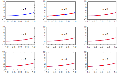
So we see that all approximations with
\( n \ge 3 \) terms give very good approximations. Now we use Chebyshev polynomials of the second kind:
\[
e^x \approx \sum_{k=0}^n b_k U_k (x) ,
\]
where
\[
b_k = \int_{-1}^1 e^x \,U_k (x)\, \sqrt{1-x^2} \, {\text d} x = 2\left( k+1 \right) I_{k+1} (1), \quad k=0,1,2,\ldots .
\]
Therefore, on the interval [-1,1], we have
\[
e^x = 2\,\sum_{k\ge 0} \left( k+1 \right) I_{k+1} (1) \, U_k (x) .
\]
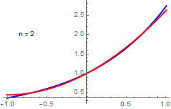
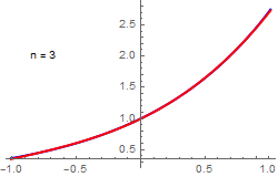
Upon plotting finite sum approximation, we see that approximation with three terms is enough. Its mean square error is about 0.0000268334.
exp[m_, x_] :=
2*Sum[(k + 1)*BesselI[k + 1, 1]*ChebyshevU[k, x], {k, 0, m}]
Exponential approximation with
N = 2 and
N = 3 terms.
■
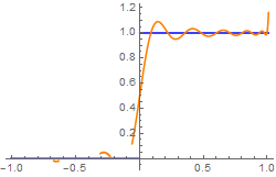
Example 4A: Heaviside function expressing through Chebyshev polynomials
Example 4A:
\[
H(t) = \frac{c_0}{2} + \sum_{k\ge 1} c_k T_k (t) .
\]
The coefficients can be evaluated explicitly:
\begin{align*}
c_0 &= \frac{2}{\pi} \, \int_0^1 \frac{{\text d}x}{\sqrt{1- x^2}} =1,
\\
c_n &= \frac{2}{\pi} \, \int_0^1 \frac{T_n (x)\,{\text d}x}{\sqrt{1- x^2}} = \left\{
\begin{array}{ll}
0 , & \ \mbox{if $n=2k$ is even} \\
(-1)^k \,\frac{2}{n\pi} , & \ \mbox{if $n = 2k+1$ is odd. }
\end{array}
\right.
\end{align*}
Therefore,
\[
H(t) = \frac{1}{2} + \frac{2}{\pi} \,\sum_{k\ge 0} \frac{(-1)^k}{2k+1}\, T_{2k+1} (t) .
\]
We plot its approximation with 11 terms:
heaviside[m_, t_] =
1/2 + (2/Pi)*
Sum[(-1)^k *ChebyshevT[2*k + 1, t]/(2*k + 1) , {k, 0, m}];
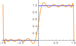
We repeat calculations with Chebyshev polynomials of the second kind:
\[
H(t) = \frac{1}{2} + \frac{4}{\pi} \, \sum_{k\ge 0} \frac{(-1)^k\, k}{(2k+1)(2k+3)}\, U_{2k+1} (t) .
\]
The following graph presents 10 term approximation with Chebyshev polynomials of second kind.
chebsum[m_] :=
1/2 - (4/Pi)*
Sum[(-1)^k *k/(2*k - 1)/(2*k + 1) *ChebyshevU[2*k - 1, t], {k, 1,
m}]
We observe Gibbs phenomenon near point of discontinuity
t = 0 in both expansions with respect to Chebyshev polynomials of the first and second kind, as well as bad convergence at end points.
■
Example 5A: Signum expansion into Chebyshev series
Example 5A:
\begin{align*}
\mbox{sign}(x) = \sum_{n\ge 1} a_n T_n (x)
= \sum_{n\ge 1} b_n U_n (x)
= \sum_{n\ge 0} c_n V_n (x)
= \sum_{n\ge 0} d_n W_n (x) ,
\end{align*}
where
\begin{align*}
a_n &= - \frac{2}{\pi} \int_{-1}^0 \frac{T_n (x)}{\sqrt{1-x^2}} \, {\text d}x +
\frac{2}{\pi} \int_0^1 \frac{T_k (x)}{\sqrt{1-x^2}} \, {\text d}x =
\frac{4}{\pi} \times \begin{cases}
\frac{1}{n} , & \ \mbox{ if $n$ is odd}, \\
0 , & \ \mbox{ if $n$ is even};
\end{cases}
\\
b_n &= - \frac{2}{\pi} \int_{-1}^0 U_n (x) \,\sqrt{1-x^2} \, {\text d}x +
\frac{2}{\pi} \int_0^1 U_n (x) \,\sqrt{1-x^2} \, {\text d}x =
\frac{8}{\pi} \times \begin{cases}
0, & \ \mbox{if $n$ is even}, \\
\frac{(-1)^k k}{(2k-1)(2k+1)} , & \ \mbox{ if $n= 2k-1$ is odd};
\end{cases}
\\
c_n &= \frac{1}{\pi} \int_0^1 \left( \frac{1+x}{1-x} \right)^{1/2} V_n (x) \,
{\text d}x - \frac{1}{\pi} \int_{-1}^0 \left( \frac{1+x}{1-x} \right)^{1/2}
V_n (x) \, {\text d}x =
\\
d_n &= \frac{1}{\pi} \int_0^1 \left( \frac{1-x}{1+x} \right)^{1/2} W_n (x) \,
{\text d}x - \frac{1}{\pi} \int_{-1}^0 \left( \frac{1+x}{1-x} \right)^{1/2}
W_n (x) \, {\text d}x =
\end{align*}
We plot partial sums using
Mathematica :
SA[x_] = (4/Pi)*Sum[ChebyshevT[2*k - 1, x]/(2*k - 1), {k, 0, 10}]
Plot[SA[x], {x, -1, 1}]
CT[n_, x_] := Piecewise[{{1, -1 < x < 0}, {0, 0}, {-1, 0 < x < 1}}];
■
Some other examples of Chebyshev expansions
Example:
\begin{align*}
\frac{1}{a^2 - x^2} &= \frac{1}{a \sqrt{a^2 -1}} \left[ 1 - 2\sum_{k\ge 1} \left( a - \sqrt{a^2 -1} \right)^{2k} T_{2k} (x) \right] , \qquad a > 1,
\\
\frac{1}{x-a} &= \frac{1}{\sqrt{a^2 -1}} + \frac{2}{\sqrt{a^2 -1}} \sum_{n\ge 1} \left( a - \sqrt{a^2 -1} \right)^{n} T_{n} (x)
\\
\mbox{sign}(x) &= -\frac{4}{\pi} \,\sum_{k \ge 1} \frac{(-1)^k}{2k-1} \,T_{2k-1} (x) ,
\\
|x| &= \frac{2}{\pi} - \frac{4}{\pi} \,\sum_{k\ge 1} \frac{(-1)^k}{4k^2 -1} \,T_{2k} (x)
\\
&= \frac{1}{2} - \sum_{k\ge 1} (-1)^k \frac{(2k-3)!!}{(2k+2)!!} \, (4k+1)\,P_{2k} (x) ,
\\
\sin ax &= J_1 (a) + 2 \sum_{k\ge 1} (-1)^k J_{2k+1} (a)\, T_{2k+1} (x) ,
\\
\sinh ax &= I_1 (a) + 2 \sum_{k\ge 1} I_{2k+1} (a) \, T_{2k+1} (x) ,
\\
\cosh ax &= I_0 (a) + 2 \sum_{k\ge 1} I_{2k} (a) \, T_{2k} (x) ,
\\
\mbox{arccos}(x) &= \frac{\pi}{2} - \frac{4}{\pi} \,\sum_{k\ge 1} \frac{1}{(2k-1)^2}\, T_{2k-1} (x) ,
\\
\mbox{arcsin}(x) &= \frac{4}{\pi} \,\sum_{k\ge 1} \frac{1}{(2k-1)^2}\, T_{2k-1} (x) .
\\
\arctan x &= 2 \sum_{k \ge 0} (-1)^k \frac{p^{2k+1}}{2k+1} \,T_{2k+1} (x) , \qquad p = \sqrt{2} -1 ,
\\
\sqrt{1-x^2} &= \frac{2}{\pi} - \frac{4}{\pi} \sum_{n\ge 1} \frac{T_{2n} (x)}{4 n^2 -1} ,
\\
\frac{1}{4}\,\ln \left( \frac{1+x}{1-x} \right) &= \sum_{n\ge 1} \frac{T_{2n -1} (x)}{2n-1} , \qquad -1 < x < 1 ,
\\
\frac{1-rx}{1 -2rx + r^2} &= \sum_{n\he 0} r^n T_n (x) , \qquad 0 \le r < 1 ,
\\
\ln \left( 1 -2rx + r^2 \right) &= -2 \sum_{n\he 1} \frac{r^n}{n}\, T_n (x) ,
\\
\ln \frac{1 + 2rx + r^2}{1 - 2rx + r^2} &= 4 \sum_{k\ge 0} \frac{r^{2k+1}}{2k+1}\,T_{2k+1} (x) .
\end{align*}
Bessel functions:
\begin{align*}
J_0 (ax) &= \sum_{k\ge 0} {\cal E}_k (-1)^k J_k^2 \left( a/2 \right) T_{2k} (x) ,
\\
J_1 (ax) &= 2 \sum_{k\ge 0} (-1)^k J_k \left( a/2 \right) T_{2k+1} (x) .1
\end{align*}
Delta function:
\[
\delta (x) = \frac{1}{\pi} + \frac{2}{\pi} \sum_{n\ge 1} (-1)^n T_{2n} (x) .
\]
■
We are tempted to expand a function into the series over Chebyshev polynomials of the second kind:
\begin{equation} \label{EqCheb2.1}
f(x) = \sum_{k\ge 0} \,b_k\, U_{k} (x ) ,
\end{equation}
where
\begin{equation} \label{EqCheb2.2}
b_k = \frac{2}{\pi}\,\int_{-1}^1 \,f(x)\, U_{k} (x )\,\sqrt{1-x^2}\, {\text d} x = \frac{2}{\pi}\,\int_{0}^{\pi} \, f\left( \cos \,\theta \right) \sin \left( (k+1)\,\theta \right) \sin \theta \,{\text d} \theta , \qquad k=0,1,2,\ldots .
\end{equation}
Formula \eqref{EqCheb2.2} show that the Chebyshev expansion with respect to Chebyshev polynomials of the second kind is actually the sine-Fourier series for the odd function
\( \displaystyle f(\cos \theta )\,\sin\theta . \)
Since U 2k+1 (0) = 0, we get the expansion of
the Dirac delta function :
\[
\delta (x) = \frac{2}{\pi}\,\sum_{k\ge 0} (-1)^k U_{2k} (x) .
\]
If function g (x ) is continuous on the interval [−1, 1] and vanish at end points so that \( g(x)/\sqrt{1-x^2} \) is quadratically/absolutely integrable on the interval, then we can expand it as
\[
g(x) = \sqrt{1-x^2} \,\sum_{k\ge 0} \,b_k\, U_{k} (x ) ,
\]
where
\[
b_k = \frac{2}{\pi}\,\int_{-1}^1 \,g(x)\, U_{k} (x )\, {\text d} x , \qquad k=0,1,2,\ldots .
\]
Example 1B: Root function
Example 1B: \( f(x) = \sqrt{1 - x^2} . \) To expand it into Chebyshev series over second kind polynomials, we need to calculate Fourier-Chebyshev coefficients according to \eqref{EqCheb2.2}:
\[
b_n = \frac{2}{\pi}\,\int_{-1}^1 \sqrt{1-x^2} \,\sqrt{1- x^2} \,U_n (x) \,{\text d}x = \frac{2}{\pi}\,\int_{-1}^1 \left( 1 - x^2 \right) U_n (x) \,{\text d}x = \frac{2}{\pi}\cdot \frac{2}{3 + n - 3n^2 - n^3} \left[ 1 + (-1)^n \right] .
\]
Indeed,
Mathematica is able to calculate this integral
Integrate[(1 - x^2)*ChebyshevU[n, x], {x, -1, 1}]
(2 + 2 Cos[n \[Pi]])/(3 + n - 3 n^2 - n^3)
Since
\[
1 + (-1)^n = \begin{cases}
2 , & \ \mbox{ if } \ n = 2k,
\\
0, & \ \mbox{ if } \ n = 2k+1 .
\end{cases}
\]
So we get
\[
\sqrt{1- x^2} = \frac{2}{\pi}\, \sum_{k\ge 0} \frac{4}{3 + 2k -12 k^2 - 8 k^3} \, U_{2k} (x) .
\]
Now we consider another root function \( g(x) = \sqrt{1 - x} . \) The corresponding Fourier--Chebyshev coefficients are evaluated according to Eq.\eqref{EqCheb2.2}:
\[
b_n = \frac{2}{\pi}\,\int_{0}^{\pi} \sin \frac{\theta}{2} \,\sin [(n+1) \theta ] \,\sin\theta \, {\text d}\theta
\]
because
\( \sqrt{1 - \cos\theta} = \sin\frac{\theta}{2} . \) We again ask
Mathematica to rescure
Integrate[Sin[t/2]*Sin[(n + 1)*t]*Sin[t], {t, 0, Pi}]
(4 (-4 (1 + n) + (1 + 8 n + 4 n^2) Sin[n \[Pi]]))/((-1 + 2 n) (1 +
2 n) (3 + 2 n) (5 + 2 n))
This yields
\[
b_n = - \frac{2}{\pi}\,\frac{16 \left( 1 + n \right)}{(4n^2 -1)(3 + 2n)(5 + 2n)} , \qquad n=0,1,2,\ldots .
\]
So the required expansion becomes
\[
\sqrt{1-x} = - \frac{2}{\pi}\,\sum_{n\ge 0} \frac{16 \left( 1 + n \right)}{(4n^2 -1)(3 + 2n)(5 + 2n)} \, U_n (x) .
\]
■
Example 4B: Heaviside function expressing through Chebyshev polynomials
Example 4B:
\[
H(t) = \frac{c_0}{2} + \sum_{k\ge 1} c_k T_k (t) .
\]
The coefficients can be evaluated explicitly:
\begin{align*}
c_0 &= \frac{2}{\pi} \, \int_0^1 \frac{{\text d}x}{\sqrt{1- x^2}} =1,
\\
c_n &= \frac{2}{\pi} \, \int_0^1 \frac{T_n (x)\,{\text d}x}{\sqrt{1- x^2}} = \left\{
\begin{array}{ll}
0 , & \ \mbox{if $n=2k$ is even} \\
(-1)^k \,\frac{2}{n\pi} , & \ \mbox{if $n = 2k+1$ is odd. }
\end{array}
\right.
\end{align*}
Therefore,
\[
H(t) = \frac{1}{2} + \frac{2}{\pi} \,\sum_{k\ge 0} \frac{(-1)^k}{2k+1}\, T_{2k+1} (t) .
\]
We plot its approximation with 11 terms:
heaviside[m_, t_] =
1/2 + (2/Pi)*
Sum[(-1)^k *ChebyshevT[2*k + 1, t]/(2*k + 1) , {k, 0, m}];
We repeat calculations with Chebyshev polynomials of the second kind:
\[
H(t) = \frac{1}{2} + \frac{4}{\pi} \, \sum_{k\ge 0} \frac{(-1)^k\, k}{(2k+1)(2k+3)}\, U_{2k+1} (t) .
\]
The following graph presents 10 term approximation with Chebyshev polynomials of second kind.
chebsum[m_] :=
1/2 - (4/Pi)*
Sum[(-1)^k *k/(2*k - 1)/(2*k + 1) *ChebyshevU[2*k - 1, t], {k, 1,
m}]
We observe Gibbs phenomenon near point of discontinuity
t = 0 in both expansions with respect to Chebyshev polynomials of the first and second kind, as well as bad convergence at end points.
■
Example 5B: Signum expansion into Chebyshev series
Example 5B:
\begin{align*}
\mbox{sign}(x) = \sum_{n\ge 1} a_n T_n (x)
= \sum_{n\ge 1} b_n U_n (x)
= \sum_{n\ge 0} c_n V_n (x)
= \sum_{n\ge 0} d_n W_n (x) ,
\end{align*}
where
\begin{align*}
a_n &= - \frac{2}{\pi} \int_{-1}^0 \frac{T_n (x)}{\sqrt{1-x^2}} \, {\text d}x +
\frac{2}{\pi} \int_0^1 \frac{T_k (x)}{\sqrt{1-x^2}} \, {\text d}x =
\frac{4}{\pi} \times \begin{cases}
\frac{1}{n} , & \ \mbox{ if $n$ is odd}, \\
0 , & \ \mbox{ if $n$ is even};
\end{cases}
\\
b_n &= - \frac{2}{\pi} \int_{-1}^0 U_n (x) \,\sqrt{1-x^2} \, {\text d}x +
\frac{2}{\pi} \int_0^1 U_n (x) \,\sqrt{1-x^2} \, {\text d}x =
\frac{8}{\pi} \times \begin{cases}
0, & \ \mbox{if $n$ is even}, \\
\frac{(-1)^k k}{(2k-1)(2k+1)} , & \ \mbox{ if $n= 2k-1$ is odd};
\end{cases}
\\
c_n &= \frac{1}{\pi} \int_0^1 \left( \frac{1+x}{1-x} \right)^{1/2} V_n (x) \,
{\text d}x - \frac{1}{\pi} \int_{-1}^0 \left( \frac{1+x}{1-x} \right)^{1/2}
V_n (x) \, {\text d}x =
\\
d_n &= \frac{1}{\pi} \int_0^1 \left( \frac{1-x}{1+x} \right)^{1/2} W_n (x) \,
{\text d}x - \frac{1}{\pi} \int_{-1}^0 \left( \frac{1+x}{1-x} \right)^{1/2}
W_n (x) \, {\text d}x =
\end{align*}
We plot partial sums using
Mathematica :
SA[x_] = (4/Pi)*Sum[ChebyshevT[2*k - 1, x]/(2*k - 1), {k, 0, 10}]
Plot[SA[x], {x, -1, 1}]
CT[n_, x_] := Piecewise[{{1, -1 < x < 0}, {0, 0}, {-1, 0 < x < 1}}];
■
A function
f (
x ) that satisfies the Dirichlet conditions on the interval [−1, 1] can be expanded into Chebyshev series
\begin{equation} \label{EqCheb3.1}
f(x) = \sum_{k\ge 0} \,c_k\, V_{k} (x ) , \qquad -1 < x < 1 ,
\end{equation}
where
\begin{equation} \label{EqCheb3.2}
c_k = \frac{1}{\pi}\,\int_{-1}^1 \,f(x)\, V_{k} (x )\left( \frac{1+x}{1-x} \right)^{1/2} {\text d} x , \qquad k=0,1,2,\ldots .
\end{equation}
In the integral, we make substitution
\( x = \cos \theta \quad \Longrightarrow \quad {\text d}x = -\sin\theta\,{\text d}\theta . \) The radical becomes
\[
\left( \frac{1+x}{1-x} \right)^{1/2} = \frac{1+x}{\sqrt{1 - x^2}} = \frac{1 + \cos\theta}{\sin\theta} = \frac{2\,\cos^2 \frac{\theta}{2}}{\sin\theta} .
\]
The Chebyshev polynomial of the third kind in new variable θ is the ratio:
\[
V_n (\cos \theta ) = \frac{\cos \left( \frac{2n+1}{2}\,\theta \right)}{\cos \left( \frac{\theta}{2} \right)} .
\]
Therefore, the kernel of the Fourier--Chebyshev coefficient is the product of these expressions:
\[
C_n = \frac{1 + \cos\theta}{\sin\theta} \cdot \frac{\cos \left( \frac{2n+1}{2}\,\theta \right)}{\cos \left( \frac{\theta}{2} \right)} \cdot \sin\theta = 2\,\cos \left( \frac{\theta}{2} \right) \cdot \cos \left( \frac{2n+1}{2}\,\theta \right)
\]
because
\( 1 + \cos \theta = 2\,\cos^2 \frac{\theta}{2} . \) We replace the product of two cosine functions with the sum:
\[
2\,\cos\alpha\,\cos\beta = \cos \left( \alpha + \beta \right) + \cos \left( \alpha - \beta \right) .
\]
This yields
\begin{equation} \label{EqCheb3.3}
c_n = \frac{1}{\pi}\,\int_{0}^{\pi} \,f(\cos\theta )\left[ \cos n\theta + \cos (n+1)\theta \right] {\text d} \theta , \qquad n=0,1,2,\ldots .
\end{equation}
This formula shows that the coefficient c n is the average of two ajacent coefficients of cosine Fourier series for the even function f (cosθ).
Example 1C: Root function
Example 1C: \( f(x) = \sqrt{1 - x^2} . \) To expand it into Chebyshev series over third kind polynomials, we need to calculate Fourier-Chebyshev coefficients according to \eqref{EqCheb3.3}:
\[
c_n = \frac{1}{\pi}\,\int_{0}^{\pi} \sqrt{1-\cos^2 \theta} \left[ \cos n\theta + \cos (n+1)\theta \right] {\text d} \theta = \frac{(-1)^n -1}{n(2+n)} + \frac{1 + (-1)^n}{1 - n^2} .
\]
Indeed,
Mathematica is able to calculate this integral
Integrate[ Sin[t]*(Cos[n*t] + Cos[(n + 1)*t]), {t, 0, Pi}
(-1 + Cos[n \[Pi]])/(n (2 + n)) + (1 + Cos[n \[Pi]])/(1 - n^2)
Since
\[
1 + (-1)^n = \begin{cases}
2 , & \ \mbox{ if } \ n = 2k,
\\
0, & \ \mbox{ if } \ n = 2k+1 ;
\end{cases} \qquad \mbox{and} \qquad (-1)^n -1 = \begin{cases}
\phantom{-}0 , & \ \mbox{ if } \ n = 2k,
\\
-2, & \ \mbox{ if } \ n = 2k+1 .
\end{cases}
\]
So we get
\[
\sqrt{1- x^2} = \frac{2}{\pi}\, \sum_{k\ge 0} \frac{1}{1 - 4 k^2} \, V_{2k} (x) - \frac{2}{\pi}\, \sum_{k\ge 0} \frac{1}{(2k+1)(3+2k)}\, V_{2k+1} (x) .
\]
Now we consider another root function \( g(x) = \sqrt{1 - x} . \) The corresponding Fourier--Chebyshev coefficients are evaluated according to Eq.\eqref{EqCheb2.2}:
\[
b_n = \frac{2}{\pi}\,\int_{0}^{\pi} \sin \frac{\theta}{2} \,\sin [(n+1) \theta ] \,\sin\theta \, {\text d}\theta
\]
because
\( \sqrt{1 - \cos\theta} = \sin\frac{\theta}{2} . \) We again ask
Mathematica to rescue
Integrate[Sin[t/2]*Sin[(n + 1)*t]*Sin[t], {t, 0, Pi}]
(4 (-4 (1 + n) + (1 + 8 n + 4 n^2) Sin[n \[Pi]]))/((-1 + 2 n) (1 +
2 n) (3 + 2 n) (5 + 2 n))
This yields
\[
b_n = - \frac{2}{\pi}\,\frac{16 \left( 1 + n \right)}{(4n^2 -1)(3 + 2n)(5 + 2n)} , \qquad n=0,1,2,\ldots .
\]
So the required expansion becomes
\[
\sqrt{1-x} = - \frac{2}{\pi}\,\sum_{n\ge 0} \frac{16 \left( 1 + n \right)}{(4n^2 -1)(3 + 2n)(5 + 2n)} \, U_n (x) .
\]
■
Example 4C: Heaviside function expressing through Chebyshev polynomials
Example 4C:
\[
H(t) = \frac{c_0}{2} + \sum_{k\ge 1} c_k T_k (t) .
\]
The coefficients can be evaluated explicitly:
\begin{align*}
c_0 &= \frac{2}{\pi} \, \int_0^1 \frac{{\text d}x}{\sqrt{1- x^2}} =1,
\\
c_n &= \frac{2}{\pi} \, \int_0^1 \frac{T_n (x)\,{\text d}x}{\sqrt{1- x^2}} = \left\{
\begin{array}{ll}
0 , & \ \mbox{if $n=2k$ is even} \\
(-1)^k \,\frac{2}{n\pi} , & \ \mbox{if $n = 2k+1$ is odd. }
\end{array}
\right.
\end{align*}
Therefore,
\[
H(t) = \frac{1}{2} + \frac{2}{\pi} \,\sum_{k\ge 0} \frac{(-1)^k}{2k+1}\, T_{2k+1} (t) .
\]
We plot its approximation with 11 terms:
heaviside[m_, t_] =
1/2 + (2/Pi)*
Sum[(-1)^k *ChebyshevT[2*k + 1, t]/(2*k + 1) , {k, 0, m}];
We repeat calculations with Chebyshev polynomials of the second kind:
\[
H(t) = \frac{1}{2} + \frac{4}{\pi} \, \sum_{k\ge 0} \frac{(-1)^k\, k}{(2k+1)(2k+3)}\, U_{2k+1} (t) .
\]
The following graph presents 10 term approximation with Chebyshev polynomials of second kind.
chebsum[m_] :=
1/2 - (4/Pi)*
Sum[(-1)^k *k/(2*k - 1)/(2*k + 1) *ChebyshevU[2*k - 1, t], {k, 1,
m}]
We observe Gibbs phenomenon near point of discontinuity
t = 0 in both expansions with respect to Chebyshev polynomials of the first and second kind, as well as bad convergence at end points.
■
Example 5C: Signum expansion into Chebyshev series
Example 5C:
\begin{align*}
\mbox{sign}(x) = \sum_{n\ge 1} a_n T_n (x)
= \sum_{n\ge 1} b_n U_n (x)
= \sum_{n\ge 0} c_n V_n (x)
= \sum_{n\ge 0} d_n W_n (x) ,
\end{align*}
where
\begin{align*}
a_n &= - \frac{2}{\pi} \int_{-1}^0 \frac{T_n (x)}{\sqrt{1-x^2}} \, {\text d}x +
\frac{2}{\pi} \int_0^1 \frac{T_k (x)}{\sqrt{1-x^2}} \, {\text d}x =
\frac{4}{\pi} \times \begin{cases}
\frac{1}{n} , & \ \mbox{ if $n$ is odd}, \\
0 , & \ \mbox{ if $n$ is even};
\end{cases}
\\
b_n &= - \frac{2}{\pi} \int_{-1}^0 U_n (x) \,\sqrt{1-x^2} \, {\text d}x +
\frac{2}{\pi} \int_0^1 U_n (x) \,\sqrt{1-x^2} \, {\text d}x =
\frac{8}{\pi} \times \begin{cases}
0, & \ \mbox{if $n$ is even}, \\
\frac{(-1)^k k}{(2k-1)(2k+1)} , & \ \mbox{ if $n= 2k-1$ is odd};
\end{cases}
\\
c_n &= \frac{1}{\pi} \int_0^1 \left( \frac{1+x}{1-x} \right)^{1/2} V_n (x) \,
{\text d}x - \frac{1}{\pi} \int_{-1}^0 \left( \frac{1+x}{1-x} \right)^{1/2}
V_n (x) \, {\text d}x =
\\
d_n &= \frac{1}{\pi} \int_0^1 \left( \frac{1-x}{1+x} \right)^{1/2} W_n (x) \,
{\text d}x - \frac{1}{\pi} \int_{-1}^0 \left( \frac{1+x}{1-x} \right)^{1/2}
W_n (x) \, {\text d}x =
\end{align*}
We plot partial sums using
Mathematica :
SA[x_] = (4/Pi)*Sum[ChebyshevT[2*k - 1, x]/(2*k - 1), {k, 0, 10}]
Plot[SA[x], {x, -1, 1}]
CT[n_, x_] := Piecewise[{{1, -1 < x < 0}, {0, 0}, {-1, 0 < x < 1}}];
■
A function
f (
x ) that satisfies the Dirichlet conditions on the interval [−1, 1] can be expanded into Chebyshev series
\begin{equation} \label{EqCheb4.1}
f(x) = \sum_{k\ge 0} \,d_k\, W_{k} (x ) , \qquad -1 < x < 1 ,
\end{equation}
where
\begin{equation} \label{EqCheb4.2}
d_k = \frac{1}{\pi}\,\int_{-1}^1 \,f(x)\, W_{k} (x )\left( \frac{1-x}{1+x} \right)^{1/2} {\text d} x , \qquad k=0,1,2,\ldots .
\end{equation}
Using expression
\[
W_n (\cos \theta ) = \frac{\sin \left( \frac{2n+1}{2}\,\theta \right)}{\sin \left( \frac{\theta}{2} \right)}
\]
we rewrite the kernel of coefficient \eqref{EqCheb4.2} as
\[
D_n = \frac{\sin\theta}{1 + \cos\theta} \cdot \frac{\sin \left( \frac{2n+1}{2}\,\theta \right)}{\sin \left( \frac{\theta}{2} \right)} \cdot \sin\theta = \frac{\sin\theta}{\cos^2 \frac{\theta}{2}} \cdot \frac{\sin \left( \frac{2n+1}{2}\,\theta \right)}{\sin \left( \frac{\theta}{2} \right)} \cdot \sin\theta = 2\,\sin \left( \frac{\theta}{2} \right) \sin \left( \frac{2n+1}{2}\,\theta \right) .
\]
This allows us to rewrite the coefficient
d n as
\begin{equation} \label{EqCheb4.3}
d_k = \frac{1}{\pi}\,\int_{-1}^1 \,f(\cos\theta )\left[ \cos n\theta - \cos [(n+1) \theta ] \right] {\text d}\theta , \qquad n=0,1,2,\ldots .
\end{equation}
Example 1D: Root function
Example 1D: \( f(x) = \sqrt{1 - x^2} . \) To expand it into Chebyshev series over second kind polynomials, we need to calculate Fourier-Chebyshev coefficients according to \eqref{EqCheb2.2}:
\[
b_n = \frac{2}{\pi}\,\int_{-1}^1 \sqrt{1-x^2} \,\sqrt{1- x^2} \,U_n (x) \,{\text d}x = \frac{2}{\pi}\,\int_{-1}^1 \left( 1 - x^2 \right) U_n (x) \,{\text d}x = \frac{2}{\pi}\cdot \frac{2}{3 + n - 3n^2 - n^3} \left[ 1 + (-1)^n \right] .
\]
Indeed,
Mathematica is able to calculate this integral
Integrate[(1 - x^2)*ChebyshevU[n, x], {x, -1, 1}]
(2 + 2 Cos[n \[Pi]])/(3 + n - 3 n^2 - n^3)
Since
\[
1 + (-1)^n = \begin{cases}
2 , & \ \mbox{ if } \ n = 2k,
\\
0, & \ \mbox{ if } \ n = 2k+1 .
\end{cases}
\]
So we get
\[
\sqrt{1- x^2} = \frac{2}{\pi}\, \sum_{k\ge 0} \frac{4}{3 + 2k -12 k^2 - 8 k^3} \, U_{2k} (x) .
\]
Now we consider another root function \( g(x) = \sqrt{1 - x} . \) The corresponding Fourier--Chebyshev coefficients are evaluated according to Eq.\eqref{EqCheb2.2}:
\[
b_n = \frac{2}{\pi}\,\int_{0}^{\pi} \sin \frac{\theta}{2} \,\sin [(n+1) \theta ] \,\sin\theta \, {\text d}\theta
\]
because
\( \sqrt{1 - \cos\theta} = \sin\frac{\theta}{2} . \) We again ask
Mathematica to rescure
Integrate[Sin[t/2]*Sin[(n + 1)*t]*Sin[t], {t, 0, Pi}]
(4 (-4 (1 + n) + (1 + 8 n + 4 n^2) Sin[n \[Pi]]))/((-1 + 2 n) (1 +
2 n) (3 + 2 n) (5 + 2 n))
This yields
\[
b_n = - \frac{2}{\pi}\,\frac{16 \left( 1 + n \right)}{(4n^2 -1)(3 + 2n)(5 + 2n)} , \qquad n=0,1,2,\ldots .
\]
So the required expansion becomes
\[
\sqrt{1-x} = - \frac{2}{\pi}\,\sum_{n\ge 0} \frac{16 \left( 1 + n \right)}{(4n^2 -1)(3 + 2n)(5 + 2n)} \, U_n (x) .
\]
■
Example 4D: Heaviside function expressing through Chebyshev polynomials
Example 4D:
\[
H(t) = \frac{c_0}{2} + \sum_{k\ge 1} c_k T_k (t) .
\]
The coefficients can be evaluated explicitly:
\begin{align*}
c_0 &= \frac{2}{\pi} \, \int_0^1 \frac{{\text d}x}{\sqrt{1- x^2}} =1,
\\
c_n &= \frac{2}{\pi} \, \int_0^1 \frac{T_n (x)\,{\text d}x}{\sqrt{1- x^2}} = \left\{
\begin{array}{ll}
0 , & \ \mbox{if $n=2k$ is even} \\
(-1)^k \,\frac{2}{n\pi} , & \ \mbox{if $n = 2k+1$ is odd. }
\end{array}
\right.
\end{align*}
Therefore,
\[
H(t) = \frac{1}{2} + \frac{2}{\pi} \,\sum_{k\ge 0} \frac{(-1)^k}{2k+1}\, T_{2k+1} (t) .
\]
We plot its approximation with 11 terms:
heaviside[m_, t_] =
1/2 + (2/Pi)*
Sum[(-1)^k *ChebyshevT[2*k + 1, t]/(2*k + 1) , {k, 0, m}];
We repeat calculations with Chebyshev polynomials of the second kind:
\[
H(t) = \frac{1}{2} + \frac{4}{\pi} \, \sum_{k\ge 0} \frac{(-1)^k\, k}{(2k+1)(2k+3)}\, U_{2k+1} (t) .
\]
The following graph presents 10 term approximation with Chebyshev polynomials of second kind.
chebsum[m_] :=
1/2 - (4/Pi)*
Sum[(-1)^k *k/(2*k - 1)/(2*k + 1) *ChebyshevU[2*k - 1, t], {k, 1,
m}]
We observe Gibbs phenomenon near point of discontinuity
t = 0 in both expansions with respect to Chebyshev polynomials of the first and second kind, as well as bad convergence at end points.
■
Example 5D: Signum expansion into Chebyshev series
Example 5D:
\begin{align*}
\mbox{sign}(x) = \sum_{n\ge 1} a_n T_n (x)
= \sum_{n\ge 1} b_n U_n (x)
= \sum_{n\ge 0} c_n V_n (x)
= \sum_{n\ge 0} d_n W_n (x) ,
\end{align*}
where
\begin{align*}
a_n &= - \frac{2}{\pi} \int_{-1}^0 \frac{T_n (x)}{\sqrt{1-x^2}} \, {\text d}x +
\frac{2}{\pi} \int_0^1 \frac{T_k (x)}{\sqrt{1-x^2}} \, {\text d}x =
\frac{4}{\pi} \times \begin{cases}
\frac{1}{n} , & \ \mbox{ if $n$ is odd}, \\
0 , & \ \mbox{ if $n$ is even};
\end{cases}
\\
b_n &= - \frac{2}{\pi} \int_{-1}^0 U_n (x) \,\sqrt{1-x^2} \, {\text d}x +
\frac{2}{\pi} \int_0^1 U_n (x) \,\sqrt{1-x^2} \, {\text d}x =
\frac{8}{\pi} \times \begin{cases}
0, & \ \mbox{if $n$ is even}, \\
\frac{(-1)^k k}{(2k-1)(2k+1)} , & \ \mbox{ if $n= 2k-1$ is odd};
\end{cases}
\\
c_n &= \frac{1}{\pi} \int_0^1 \left( \frac{1+x}{1-x} \right)^{1/2} V_n (x) \,
{\text d}x - \frac{1}{\pi} \int_{-1}^0 \left( \frac{1+x}{1-x} \right)^{1/2}
V_n (x) \, {\text d}x =
\\
d_n &= \frac{1}{\pi} \int_0^1 \left( \frac{1-x}{1+x} \right)^{1/2} W_n (x) \,
{\text d}x - \frac{1}{\pi} \int_{-1}^0 \left( \frac{1+x}{1-x} \right)^{1/2}
W_n (x) \, {\text d}x =
\end{align*}
We plot partial sums using
Mathematica :
SA[x_] = (4/Pi)*Sum[ChebyshevT[2*k - 1, x]/(2*k - 1), {k, 0, 10}]
Plot[SA[x], {x, -1, 1}]
CT[n_, x_] := Piecewise[{{1, -1 < x < 0}, {0, 0}, {-1, 0 < x < 1}}];
■
Clenshaw's method for the evaluation of a Chebyshev sum
References
Clenshaw, C.W., Norton, H.J.: The solution of nonlinear ordinary differential equations in chebyshev series. The Computer Journal , 1963, {\bf 6}, Issue 1, 88–92; https://doi.org/10.1093
Schweizer, W., Special Functions in Physics with MATLAB, 2021, Springer. https://link.springer.com/chapter/10.1007%2F978-3-030-64232-7_18
Return to Mathematica page main page (APMA0340) Part 1 Matrix Algebra Part 2 Linear Systems of Ordinary Differential Equations Part 3 Non-linear Systems of Ordinary Differential Equations Part 4 Numerical Methods Part 5 Fourier Series Part 6 Partial Differential EquationsPart 7 Special Functions