Return to computing page for the first course APMA0330
Return to computing page for the second course APMA0340
Return to Mathematica tutorial for the first course APMA0330
Return to Mathematica tutorial for the second course APMA0340
Return to the main page for the first course APMA0330
Return to the main page for the second course APMA0340
Return to Part I of the course APMA0340
Introduction to Linear Algebra with Mathematica

Preface


This section presents some famous expansions involving Bessel functions of the first kind, commonly denoted by Jν(x). There are several variations of these expansions and all of them are very important in applications. They are used to represent a bounded function on a finite interval (0, ℓ) (where ℓ < ∞ is a positive number) as a convergent series over a set of Bessel functions of the first kind

\[ f(x) \sim \sum_{n\ge 1} c_n J_{\nu} \left( \alpha_n x \right) , \]
where {αn}n≥1 is a particular sequence of real numbers depending on the boundary condition at the right end x = ℓ.

There are known three typical types of boundary conditions:

  • Dirichlet boundary conditions (or boundary conditions of the first kind): \( y(\ell ) =0 \qquad \Longrightarrow \qquad J_{\nu} (\alpha \ell ) =0. \)
  • Neumann boundary conditions (or boundary conditions of the second kind): \( y'(\ell ) =0 \qquad \Longrightarrow \qquad J_{\nu}' (\alpha \ell ) =0. \)
  • Boundary conditions of third kind: \( h\,y(\ell ) + y' (\ell )=0 \qquad \Longrightarrow \qquad h\,J_{\nu} (\alpha \ell ) + \alpha \,J_{\nu}' (\alpha \ell ) =0. \)

Bessel functions by itself are eigenfunctions of the singular Sturm--Liouville problem on semi-infinite interval

\[ \frac{\text d}{{\text d}x} \left( x\,\frac{{\text d}y}{{\text d}x} \right) + x\,y (x) = \lambda \left( \frac{1}{x} \right) y , \qquad y(+0) < \infty , \quad y(+\infty ) < \infty . \]
Without any loss of generality, the boundary conditions at two end points can be extended on whole semi-infinite interval (0, ∞) when the Bessel differential operator \( L\left[ x, \texttt{D} \right] = \texttt{D}\,x\,\texttt{D} + x\, \texttt{I} , \) where \( \texttt{D} = {\text d}/{\text d}x, \quad \) and \( \quad \texttt{I} = \texttt{D}^0 \) is identity operator, acts on the set of all smooth bounded functions. Upon multiplication by x the Bessel differential operator, we get a differential equation in standard Frobenius form:
\[ x^2 y'' + x\, y' + x^2 y = \lambda\, y , \qquad \mbox{subject $y(x)$ is continuous and bounded on } \quad (0, \infty ). \]
It turns out that this singular Sturm--Liouville problem has a continuous spectrum of nonnegative eigenvalues that are a custom to denote by
\[ \lambda = \nu^2 \in [0, \infty ). \]
Solutions of these equations were obtained in the Frobenius series form in section of tutorial I:
\[ J_{\nu} (x) = \left( \frac{x}{2} \right)^{\nu} \sum_{k\ge 0} \frac{(-1)^k x^{2k}}{4^k k! \Gamma (k+\nu +1)} , \]
where Γ is the Gamma function of Euler. The series above (which converges for all real or complex x) defines the Bessel function of the first kind. More comprehensive treatment of Bessel functions is given in section of Part VII.


Orthogonality of Bessel's functions


Since expansions over Bessel functions depends on their orthogonality, we recall the basic formula that was derived in section of Part VII. Let α and β be arbitrary positive real numbers. Then for ν > −1, we have
\begin{equation} \label{EqOrtho.1} \left( \alpha^2 - \beta^2 \right) \int_0^{\ell} J_{\nu} \left( \alpha\,x \right) J_{\nu} \left( \beta\,x \right) x\,{\text d} x = \ell \left[ \alpha \,J'_{\nu} \left( \alpha\,\ell \right) J_{\nu} \left( \beta\,\ell \right) - \beta\, J'_{\nu} \left( \beta\,\ell \right) ,J_{\nu} \left( \alpha\,\ell \right) \right] , \qquad \nu >' -1. \end{equation}


Bessel--Fourier Series


Let us consider a set S of bounded variation functions on an interval (0, ℓ) that vanish at right end f(ℓ) = 0. Due to oscillating behavior of Bessel's functions with real index ν, the functions Jν(x) and its derivatives have an infinite number of real zeroes, all of which are simple with the possible exception of x = 0. For nonnegative ν, we denote the n-th positive zero of the Bessel function by \( \mu_{\nu , n} , \) so

\begin{equation} \label{EqDirichlet.1} J_{\nu} \left( \mu_{\nu , n} \right) = 0 , \qquad n=1,2,3,\ldots . \end{equation}
Recall that a function f(x) is said to have a simple zero at x = μ if f(μ) = 0, but its first derivative does not vanish at this point. When index ν is fixed, we will drop it. Then the set of zeroes of Eq.\eqref{EqDirichlet.1} can be used to represent a function as the infinite series.

The Fourier--Bessel series of a function f(x) of bounded variation, defined on an interval (0, ℓ), has a representation as infinite series

\begin{equation} \label{EqDirichlet.2} \frac{f (x+0) + f(x-0)}{2} = \sum_{n \ge 1} c_n J_{\nu} \left( \mu_{\nu , n} \,\frac{x}{\ell} \right) , \end{equation}
where
\begin{equation} \label{EqDirichlet.3} c_n = \frac{2}{\ell^2 J^2_{\nu +1} (\mu_{\nu , n} )} \, \int_0^{\ell} x\,f(x)\, J_{\nu} \left( \mu_{\nu , n} \frac{x}{\ell} \right) {\text d}x, \qquad n=1,2,\ldots . \end{equation}
Indeed, from Eq.\eqref{EqOrtho.1}, it follows that for ν > −1, we have
\begin{equation} \label{EqDirichlet.4} \int_0^{\ell} J_{\nu} \left( \mu_{\nu , n} \frac{x}{\ell} \right) J_{\nu} \left( \mu_{\nu , k} \frac{x}{\ell} \right) x\,{\text d}x = \begin{cases} 0 , & \ \mbox{ if } \quad n \ne k , \\ \frac{\ell^2}{2} \,J_{\nu +1}^2 \left( \mu_{\nu , n} \right) , & \ \mbox{ if } \quad n=k. \end{cases} \end{equation}
Therefore, the norm squared of Bessel's function is
\[ \left\| J_{\nu} \left( \mu_{\nu , n} \frac{x}{\ell} \right) \right\|^2 = \left\langle J_{\nu} \left( \mu_{\nu , n} \frac{x}{\ell} \right) , J_{\nu} \left( \mu_{\nu , n} \frac{x}{\ell} \right) \right\rangle = \int_0^{\ell} J_{\nu}^2 \left( \mu_{\nu , n} \frac{x}{\ell} \right) x\,{\text d}x = \frac{\ell^2}{2} \,J_{\nu +1}^2 \left( \mu_{\nu , n} \right) . \]

Since the Fourier--Bessel series \eqref{EqDirichlet.2} exists for a piecewise continuous function that may have finite jumps at some discrete number of points, we expect to observe the Gibbs phenomenon in neighborhoods of points of discontinuity. In order to eliminate this unwanted feature, you may want to apply the Cesàro summation (also known as the Cesàro mean):

\begin{equation} \label{EqDirichlet.5} \frac{f (x+0) + f(x-0)}{2} = \lim_{N\to \infty} \,\sum_{n=1}^N \left( 1 - \frac{n-1}{N} \right) c_n J_{\nu} \left( \mu_{\nu , n} \,\frac{x}{\ell} \right) . \end{equation}
  1. Dirichlet boundary conditions: \( y(\ell ) =0 \qquad \Longrightarrow \qquad J_{\nu} (\alpha \ell ) =0. \)
    \[ c_n = \frac{2}{\ell^2 J^2_{\nu +1} (\alpha_n \ell )} \, \int_0^{\ell} x\,f(x)\, J_{\nu} (\alpha_n x)\,{\text d}x, \qquad n=1,2,\ldots . \]
  2. Neumann boundary conditions: \( y'(\ell ) =0 \qquad \Longrightarrow \qquad J_{\nu}' (\alpha \ell ) =0. \)
    \[ c_n = \frac{2}{\ell^2 J^2_{\nu} (\alpha_n \ell )} \, \int_0^{\ell} x\,f(x)\, J_{\nu} (\alpha_n x)\,{\text d}x, \qquad n=1,2,\ldots . \]
  3. Boundary conditions of third kind: \( h\,y(\ell ) + y' (\ell )=0 \qquad \Longrightarrow \qquad h\,J_{\nu} (\alpha \ell ) + \alpha \,J_{\nu}' (\alpha \ell ) =0. \)
    \[ c_n = \frac{2\alpha_n^2}{\left( \ell^2 \alpha_n^2 -\nu^2 +h \right) J^2_{\nu} (\alpha_n \ell )} \, \int_0^{\ell} x\,f(x)\, J_{\nu} (\alpha_n x)\,{\text d}x, \qquad n=1,2,\ldots . \]
If the Fourier series of f converges at the point x, then the Fourier--Bessel series of f converges to the same value at the same point.

Example 1: 
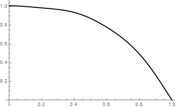
Consider the function \( f(x) = 1- x^3 \) on the interval [0,1]. Suppose we want to approximate this functions by Bessel polynomial associated with the roots from the Dirichlet boundary conditions.

First, we find the roots of the Bessel function of order 0:

zeros = N[BesselJZero[0, Range[50]]]
Out[10]=
{2.40483, 5.52008, 8.65373, 11.7915, 14.9309, 18.0711, 21.2116, \
24.3525, 27.4935, 30.6346, 33.7758, 36.9171, 40.0584, 43.1998, \
46.3412, 49.4826, 52.6241, 55.7655, 58.907, 62.0485, 65.19, 68.3315, \
71.473, 74.6145, 77.756, 80.8976, 84.0391, 87.1806, 90.3222, 93.4637, \
96.6053, 99.7468, 102.888, 106.03, 109.171, 112.313, 115.455, \
118.596, 121.738, 124.879, 128.021, 131.162, 134.304, 137.446, \
140.587, 143.729, 146.87, 150.012, 153.153, 156.295}

Table of square norms of the Bessel functions:

Table[(BesselJ[1, zeros[[k]]])^2 /2, {k, 1, 10}]
Out[2]= {0.134757, 0.0578901, 0.0368432, 0.0270188, 0.0213307, 0.0176211, \ 0.0150105, 0.0130737, 0.0115796, 0.0103919}
For the function \( f(x) = 1-x^3, \) we calculates its Fourier--Bessel approximation with N=5 terms:
sum0[x_] =
Sum[2/(BesselJ[1, zeros[[k]]])^2*BesselJ[0, x*zeros[[k]]]*
NIntegrate[x*BesselJ[0, x*zeros[[k]]]*(1 - x^3), {x, 0, 1}], {k, 1,
5}]
Out[3]=
1.27215 BesselJ[0, 2.40483 x] - 0.334787 BesselJ[0, 5.52008 x] +
0.0959387 BesselJ[0, 8.65373 x] - 0.0483534 BesselJ[0, 11.7915 x] +
0.025496 BesselJ[0, 14.9309 x]

Then we calculate its mean square error:

NIntegrate[((1 - x^3) - sum0[x])^2 , {x, 0, 1}]
Out[4]= 0.000018408

and plot

Plot[sum0[x], {x, 0, 1}, PlotStyle -> {Thick, Black}]

Next we repeat the same Fourier--Bessel approximation using the Bessel function of order 1.

zeros1 = N[BesselJZero[1, Range[50]]]
Out[6]=
{3.83171, 7.01559, 10.1735, 13.3237, 16.4706, 19.6159, 22.7601, \
25.9037, 29.0468, 32.1897, 35.3323, 38.4748, 41.6171, 44.7593, \
47.9015, 51.0435, 54.1856, 57.3275, 60.4695, 63.6114, 66.7532, \
69.8951, 73.0369, 76.1787, 79.3205, 82.4623, 85.604, 88.7458, \
91.8875, 95.0292, 98.171, 101.313, 104.454, 107.596, 110.738, \
113.879, 117.021, 120.163, 123.304, 126.446, 129.588, 132.729, \
135.871, 139.013, 142.154, 145.296, 148.438, 151.579, 154.721, \
157.863}
Table[(BesselJ[2, zeros1[[k]]])^2 /2, {k, 1, 10}]
Out[7]=
{0.0811076, 0.0450347, 0.0311763, 0.0238404, 0.0192993, 0.0162114, \
0.0139753, 0.0122814, 0.0109536, 0.009885}
sum1[x_] =
Sum[2/(BesselJ[2, zeros1[[k]]])^2*BesselJ[1, x*zeros1[[k]]]*
NIntegrate[x*BesselJ[1, x*zeros1[[k]]]*(1 - x^3), {x, 0, 1}], {k,
1, 5}]
Out[8]=
1.6444 BesselJ[1, 3.83171 x] + 0.00715804 BesselJ[1, 7.01559 x] +
0.717818 BesselJ[1, 10.1735 x] - 0.104772 BesselJ[1, 13.3237 x] +
0.503362 BesselJ[1, 16.4706 x]
NIntegrate[((1 - x^3) - sum1[x])^2 , {x, 0, 1}]
Out[9]=
0.0493142
Plot[sum1[x], {x, 0, 1}, PlotStyle -> {Thick, Black}]
This approximation cannot be good in the neighborhood of the origin because the given function is 1 at end point x = 0 but the Bessel function of order 1 is zero: \( J_1 (0) =0. \)

Example 2: 
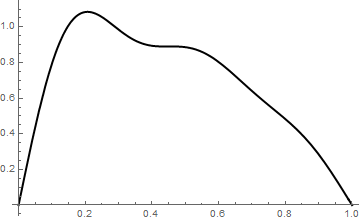
Let us consider the function \( f(x) = x(3-x)^2 \) on the interval [0,3]. This function satisfies the homogeneous Neumann condition at right end point x = 3 and the homogeneous Dirichlet condition at the origin. We expand the function into two Bessel series with respect to Bessel function of order zero and 2:

\begin{align*} x(3-x)^2 &= a_0 + \sum_{n\ge 1} a_n \,J_0 \left( \alpha_n \,\frac{x}{3} \right) , \\ x(3-x)^2 &= b_0 + \sum_{n\ge 1} b_n \,J_2 \left( \beta_n \,\frac{x}{3} \right) , \end{align*}
where αn are roots of the transcendent equation \( J'_0 (\alpha ) =0 \) and βn are roots of the equation \( J'_2 (\beta ) =0 . \) Hence,
\begin{align*} a_n &= \frac{2}{3^2 J_0^2 (\alpha_n )} \, \int_0^2 x(2-x)^2 \,J_0 \left( \alpha_n \,\frac{x}{3} \right) {\text d} x, \qquad n=1,2,\ldots , \\ b_n &= \frac{2}{3^2 J_2^2 (\beta_n )} \, \int_0^2 x(2-x)^2 \,J_2 \left( \beta_n \,\frac{x}{3} \right) {\text d} x, \qquad n=1,2,\ldots . \end{align*}

Example 3: Consider the shifted Heaviside function \( f(t) = H(t-1) \) on the interval [0,2]. We expand this function into Fourier--Bessel series with respect to the roots of the equation of the third kind: \( J_0 (2\alpha ) + \alpha \,J'_0 (\alpha ) =0: \)

\[ H(t-1) = \sum_{n\ge 1} c_n \, J_{0} (\alpha_n x) , \]
where
\[ c_n = \frac{2\alpha_n^2}{\left( 2^2 \alpha_n^2 +1 \right) J^2_{0} (\alpha_n 2 )} \, \int_1^{2} x\, J_{0} (\alpha_n x)\,{\text d}x, \qquad n=1,2,\ldots . \]
zeros = N [ BesselJZero [ 0, Range [ 100 ]]] sum0 [ x _] = Sum [ 2 / (( 4 ^ 2 ) * ( BesselJ [ 1, zeros 〚 k 〛]) ^ 2 ) * BesselJ [ 1, ( x * zeros 〚 k 〛) / 4 ] * NIntegrate [ x * HeavisideTheta [ x - 1 ] * BesselJ [ 1, ( x * zeros 〚 k 〛) / 4 ] , { x, 1, 4 }] , { k, 1, 10 }] sum1 [ x _] = Sum [ 2 / (( 4 ^ 2 ) * ( BesselJ [ 1, zeros 〚 k 〛]) ^ 2 ) * BesselJ [ 1, ( x * zeros 〚 k 〛) / 4 ] * NIntegrate [ x * HeavisideTheta [ x - 1 ] * BesselJ [ 1, ( x * zeros 〚 k 〛) / 4 ] , { x, 1, 4 }] , { k, 1, 25 }] sum2 [ x _] = Sum [ 2 / (( 4 ^ 2 ) * ( BesselJ [ 1, zeros 〚 k 〛]) ^ 2 ) * BesselJ [ 1, ( x * zeros 〚 k 〛) / 4 ] * NIntegrate [ x * HeavisideTheta [ x - 1 ] * BesselJ [ 1, ( x * zeros 〚 k 〛) / 4 ] , { x, 1, 4 }] , { k, 1, 50 }] Plot [ HeavisideTheta [ x - 1 ] , { x, 0, 4 } , PlotStyle → { Thick, Black }] Plot [ sum0 [ x ] , { x, 0, 4 } , PlotStyle → { Thick, Black }] Plot [ sum1 [ x ] , { x, 0, 4 } , PlotStyle → { Thick, Black }] Plot [ sum2 [ x ] , { x, 0, 4 } , PlotStyle → { Thick, Black }] NIntegrate [( HeavisideTheta [ x - 1 ] - sum0 [ x ]) ^ 2 , { x, 0, 4 }] NIntegrate [( HeavisideTheta [ x - 1 ] - sum1 [ x ]) ^ 2 , { x, 0, 4 }] NIntegrate [( HeavisideTheta [ x - 1 ] - sum2 [ x ]) ^ 2 , { x, 0, 4 }]

Example 4: We expand the shifted signum function into the Fourier--Bessel series:

\[ f(x) = \mbox{sign}(x-1) = \begin{cases} 1 , & \ \mbox{ for } \quad x > 1, \\ 0 , & \ \mbox{ when } quad x = 0, \\ -1, & \ \mbox{ for } \quad x < 1 . \end{cases} \tag{4.1} \]
Choosing ν = 0, we represent ff(x) as a convergent Bessel--Fourier series
\[ f(x) = \sum_{n\ge 1} c_n J_0 \left( \mu_n \frac{x}{3} \right) , \]
where
\[ c_n = \frac{2}{9\,J_1^2 \left( \mu_{0, n} \right)} \int_0^3 J_0 \left( \mu_n \frac{x}{3} \right) \mbox{sign}(x-1)\,x\,{\text d} x , \qquad n=1,2,\ldots . \]

Example 5: Consider the shifted Dirac delta function (which is actually is a distribution)

\[ \delta (t-a) = x\,\int_{0}^{\infty} J_{\nu} (xt) \, J_{\nu} (at)\, t{\text d}t , \qquad \Re \nu > -1, \quad x > 0, \quad a> 0. \]
The Dirac function can represented via the Airy functions:
\[ \delta (t-a) = \int_{-\infty}^{\infty} \mbox{Ai} (t-x) \, \mbox{Ai} (t-a)\, {\text d}t . \]
End of Example 5


Neumann Series


Let us consider a set S of bounded variation functions on an interval (0, ℓ) that have vanishing derivative at right end f'(ℓ) = 0. Due to oscillating behavior of Bessel's functions with real index ν, the functions Jν(x) and its derivatives have an infinite number of real zeroes, all of which are simple with the possible exception of x = 0. For nonnegative ν, we denote the n-th positive zero of the derivative of Bessel's function by \( \mu_{\nu , n} , \) so
\begin{equation} \label{EqNeumann.1} J'_{\nu} \left( \mu_{\nu , n} \right) = 0 \quad\mbox{or} \quad \lim_{x\to \mu_{\nu , n}} \frac{{\text d} J_{\nu} (x)}{{\text d}x} = 0 , \qquad n=1,2,3,\ldots . \end{equation}
For a smooth function f(x) of bounded variation, defined on an interval (0, ℓ), has a representation as infinite series
\begin{equation} \label{EqNeumann.2} f(x) = \sum_{n \ge 1} c_n J_{\nu} \left( \mu_{\nu , n} \,\frac{x}{\ell} \right) , \end{equation}
where
\begin{equation} \label{EqNeumann.3} c_n = \frac{2}{\ell^2 J^2_{\nu} (\mu_{\nu , n} )} \, \int_0^{\ell} x\,f(x)\, J_{\nu} \left( \mu_{\nu , n} \frac{x}{\ell} \right) {\text d}x, \qquad n=1,2,\ldots . \end{equation}
Indeed, from Eq.\eqref{EqOrtho.1}, it follows that for ν > −1, we have
\begin{equation} \label{EqNeumann.4} \int_0^{\ell} J_{\nu} \left( \mu_{\nu , n} \frac{x}{\ell} \right) J_{\nu} \left( \mu_{\nu , k} \frac{x}{\ell} \right) x\,{\text d}x = \begin{cases} 0 , & \ \mbox{ if } \quad n \ne k , \\ \frac{\ell^2}{2} \,J_{\nu +1}^2 \left( \mu_{\nu , n} \right) , & \ \mbox{ if } \quad n=k. \end{cases} \end{equation}
Therefore, the norm squared of Bessel's function is
\[ \left\| J_{\nu} \left( \mu_{\nu , n} \frac{x}{\ell} \right) \right\|^2 = \left\langle J_{\nu} \left( \mu_{\nu , n} \frac{x}{\ell} \right) , J_{\nu} \left( \mu_{\nu , n} \frac{x}{\ell} \right) \right\rangle = \int_0^{\ell} J_{\nu}^2 \left( \mu_{\nu , n} \frac{x}{\ell} \right) x\,{\text d}x = \frac{\ell^2}{2} \,J_{\nu}^2 \left( \mu_{\nu , n} \right) . \]

Example 6:

Example 7:

Example 8:

End of Example 8


Dini Series


Another Fourier–Bessel series, also known as Dini series, is associated with the third kind boundary conditions
\begin{equation} \label{EqDini.1} a\,f(\ell ) + b\,f' (\ell ) = 0 , \end{equation}
where 𝑎 and b are some real numbers (𝑎² + b² ≠ 0). Correspondingly, we consider a set of smooth functions on the finite interval (0, ℓ) that satisfy the boundary condition \eqref{EqDini.1}. As a primary set of functions for expansion, we choose Bessel's functions \( J_{\nu} \left( \frac{\mu}{\ell}\, x \right) , \) with a parameter μ. Substituting this function into boundary condition \eqref{EqDini.1}, we obtain
\[ a\,J_{\nu} (\mu ) + b\,\frac{\mu}{\ell}\, J'_{\nu} (\mu ) = 0 \qquad \Longleftrightarrow \qquad a \ell\,J_{\nu} (\mu ) + b\,\mu\,J'_{\nu} (\mu ) =0 . \]
To see whether the function
\[ \phi_{\nu} (\mu ) = a \ell\,J_{\nu} (\mu ) + b\,\mu\,J'_{\nu} (\mu ) \]
oscilates, we make an experiment and plot some examples of function ϕ.
a = 1; b = 2; L = 3;
phi0[s_] = a*L*BesselJ[0, s] + b*s*D[BesselJ[0, s], s];
Plot[phi0[s], {s, 0, 25}, AxesLabel -> {x, \[Phi]}, PlotLegends -> Placed["\[Nu]=0; a=1, b=2,L=3", Above], PlotStyle -> Thickness[0.01]]
phi1[s_] = a*L*BesselJ[1, s] + b*s*D[BesselJ[1, s], s];
Plot[phi1[s], {s, 0, 25}, AxesLabel -> {x, \[Phi]}, PlotLegends -> Placed["\[Nu]=1; a=1, b=2,L=3", Above], PlotStyle -> {Purple, Thickness[0.01]}]
phi1m[s_] = a*L*BesselJ[1, s] - b*s*D[BesselJ[1, s], s];
Plot[phi1m[s], {s, 0, 25}, AxesLabel -> {x, \[Phi]}, PlotLegends -> Placed["\[Nu]=1; a=1, b=-2,L=3", Above], PlotStyle -> {Black, {Black, Thickness[0.01]}]
ν = 1; 𝑎 = 1, b = −2, ℓ = 3.
                 
ν = 0; 𝑎 = 1, b = 2, ℓ = 3.       <ν = 1; 𝑎 = 1, b = 2, ℓ = 3. img src="part34-5/besselDini1b.png" width="230" height="230">            

Upon denoting by μν, n (n = 1, 2, …) the positive roots of the equation

\begin{equation} \label{EqDini.2} a \ell\,J_{\nu} (\mu ) + b\,\mu\,J'_{\nu} (\mu ) =0, \end{equation}
we get the Dini series
\begin{equation} \label{EqDini.3} f(x) \sim \sum_{n\ge 1} \gamma_n J_{\nu} \left( \frac{\mu_n}{\ell}\, x \right) , \end{equation}
where μn is the n-th zero of Eq.\eqref{EqDini.2}. The coefficients γn are given by
\begin{equation} \label{EqDini.4} \gamma_n = \frac{1}{\| J_{\nu} \|^2} \int_0^{\ell} f(x) \, J_{\nu} \left( \frac{\mu_n}{\ell}\, x \right) x\,{\text d} x \qquad (n=1,2, \ldots ), \end{equation}
where
\begin{equation} \label{EqDini.5} \| J_{\nu} \|^2 = \left\langle J_{\nu} \left( \frac{\mu_n}{\ell} \, x \right) , J_{\nu} \left( \frac{\mu_n}{\ell} \, x \right) \right\rangle = \int_0^{\ell} J_{\nu}^2 \left( \frac{\mu_n}{\ell}\, x \right) x\,{\text d} x \end{equation}

Example 9:

Example 10: Consider the shifted Heaviside function \( f(t) = H(t-1) \) on the interval [0,2]. We expand this function into Fourier--Bessel series with respect to the roots of the equation of the third kind: \( J_0 (2\alpha ) + \alpha \,J'_0 (\alpha ) =0: \)

\[ H(t-1) = \sum_{n\ge 1} c_n \, J_{0} (\alpha_n x) , \]
where
\[ c_n = \frac{2\alpha_n^2}{\left( 2^2 \alpha_n^2 +1 \right) J^2_{0} (\alpha_n 2 )} \, \int_1^{2} x\, J_{0} (\alpha_n x)\,{\text d}x, \qquad n=1,2,\ldots . \]

Example 11:

End of Example 11


Kapteyn Series


Series of the form
\begin{equation} \label{EqVector.2} f(z) = \sum_{n \ge 0} a_n J_n \left( nz \right) \end{equation}
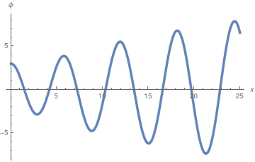
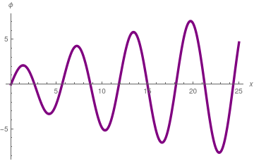
are known as Kapteyn series after the Dutch mathematician W. Kapteyn, who made the first systematic study of their properties as a function f(z) of the complex variable z ∈ ℂ. For our applications, it is sufficient to consider a real-values case, z ∈ ℝ.


  1. R. P. Boas, Jr. and Harry Pollard, Complete Sets of Bessel and Legendre Functions, Annals of Mathematics (Second Series), 1947, doi: 10.2307/1969177
  2. Courant, R. and Hilbert, D., Methods of Mathematical Physics, Wiley.
  3. Kapteyn, W., On the midpoints of integral curves of differential equations of the first degree, Nederland Akad Wetensch. Verlag, Afd. Natuurk. Nederland, 1911, 20, pp. 1446--1457 (in Dutch).
  4. Kapteyn, W., New investigations on the midpoints of integrals of differential equations of the first degree, Nederland Akad Wetensch. Verlag, Afd. Natuurk. Nederland, 1912, 20, pp. 1354--1365; 1912, 21, pp. 27--33 (in Dutch).
  5. Titchmarsh, E. C., Eigenfunction expansion associated with second order differential equations, Oxford, QA372.T45
  6. Watson, G.N., A Treatise on the Theory of Bessel Functions, Cambridge University Press; 2nd edition (August 1, 1995). ISBN-13 ‏ : ‎ 978-0521483919


Return to Mathematica page
Return to the main page (APMA0340)
Return to the Part 1 Matrix Algebra
Return to the Part 2 Linear Systems of Ordinary Differential Equations
Return to the Part 3 Non-linear Systems of Ordinary Differential Equations
Return to the Part 4 Numerical Methods
Return to the Part 5 Fourier Series
Return to the Part 6 Partial Differential Equations
Return to the Part 7 Special Functions