Preface
This section gives an introduction to modelling electric circuits.
Return to computing page for the first course APMA0330
Return to computing page for the second course APMA0340
Return to Mathematica tutorial for the first course APMA0330
Return to Mathematica tutorial for the second course APMA0340
Return to the main page for the first course APMA0330
Return to the main page for the second course APMA0340
Return to Part VI of the course APMA0340
Introduction to Linear Algebra with Mathematica
Glossary
Electric circuits
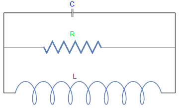
Example: Figure shows an electric circuit containing a capacitor C, a resistor R, and an inductor L, in parallel. Recall Kirchhoff's law:
- The sum of the currents flowing into any node of the system equals the sum of the currents flowing out of that node;
- The net voltage drops around each closed loop equals zero.
fbas[x_] := -(x - 2*L)/L /; L <= x < 3*L
fbas[x_] := (x - 4*L)/L /; 3*L <= x < 4*L
L = 1/2;
f[x_] := fbas[Mod[x, 4*L, -1/16^2*L]]
SetOptions[Plot, ImageSize -> 300];
resistor =
Plot[f[x], {x, -10*L, 10*L}, PlotRange -> {-1.2, 1.2},
PlotStyle -> Thickness[0.008], PlotLabel -> "R", Ticks -> None, Axes -> False]
2*Sin[t*3] - 8}, {t, 0, 5*Pi}, PlotLabel -> "L", Ticks -> None, Axes -> False, ImageSize -> Tiny]
l1 = Graphics[Line[{{-0.1, 6.7}, {-0.1, 5.3}}]]
l2 = Graphics[Line[{{0.1, 6.7}, {0.1, 5.3}}]]
l3 = Graphics[Line[{{-10, -8}, {-12, -8}, {-12, 0}, {-5, 0}}]]
l4 = Graphics[Line[{{-12, 0}, {-12.0, 6}, {-0.1, 6}}]]
l5 = Graphics[Line[{{0.1, 6}, {18, 6}, {18, -8}, {15.5619, -8}}]]
l6 = Graphics[Line[{{5, 0}, {18, 0}}]]
textC = Graphics[Text[Style["C", FontSize -> 14, Blue], {0, 7.5}]]
textR = Graphics[Text[Style["R", FontSize -> 14, Green], {0, 2.2}]]
textL = Graphics[Text[Style["L", FontSize -> 14, Red], {0.5, -5.2}]]
Show[l1, l2, l3, l4, l5, l6, resistor, Graphics[coil, PlotRegion -> {{-1, 1}, {-1, 1}}], textR, textC, textL]
Return to Mathematica page
Return to the main page (APMA0340)
Return to the Part 1 Matrix Algebra
Return to the Part 2 Linear Systems of Ordinary Differential Equations
Return to the Part 3 Non-linear Systems of Ordinary Differential Equations
Return to the Part 4 Numerical Methods
Return to the Part 5 Fourier Series
Return to the Part 6 Partial Differential Equations
Return to the Part 7 Special Functions