Return to computing page for the first course APMA0330
Return to computing page for the second course APMA0340
Return to Mathematica tutorial for the first course APMA0330
Return to Mathematica tutorial for the second course APMA0340
Return to the main page for the first course APMA0330
Return to the main page for the second course APMA0340
Return to Part III of the course APMA0340
Introduction to Linear Algebra with Mathematica
Competition modeling is one of the more challenging aspects of mathematical biology. Competition is clearly important in nature, yet there are so many ways for populations to compete that the modeling is difficult to carry out in any generality. The first general model for competition between n species was proposed by the Russian genius Andrew Kolmogorov in 1936:
His work was a generalization of the paper published by the Russian biologist Georgii Frantsevich Gause in 1934.
Since that time, the dynamic systems for modeling of competition have been studied extensively.
Such models reflect the direct impact of one population upon the other. The simplest form of competition, however, occurs when two or more populations compete for the same resource, such as a common food supply or a growth-limiting nutrient. A simple example of this type of competition can be observed in a laboratory device, called a chemostat or a continuous culture, that models competition in a very simple lake. The chemostat is a dynamic system with continuous material inputs and outputs. An ecosystem is so complex, so difficult to comprehend, that any attempt to understand its interactions is frequently doomed to failure because of a luck of rigorous controls. Consequently, in many cases we study population interactions under simplified, controllable laboratory conditions.
In this section, we explore application of two- and higher-dimensional systems of differential equations in some problems of population dynamics. We start with populations of two species that occupy the same habitat and compete for
limited resources. Although the equations we start with are extremely simple compared to the very complex relationships that exist in nature, it allows us to get some insights into ecological problems. A number of mathematical models have been constructed to address this issue.
Recall from the first part of the tutorial the logistic equation for a single species:
where r is the growth (birth) rate, and K the carrying capacity. We assume that populations of two species varies continuously and use letters x(t) and y(t) to represent their populations at time t. For these two species living in the same habitat, each of them tends to diminish the available resources for the other. In effect, they reduce each other's growth rates and saturation populations. The simplest model for reducing growth rate of species, say x, due to the presence of species y is toe replace the growth rate factor (1 - N/K) in the logistic equation by the following expressions:
\[
\begin{split}
\dot{x} &= x \left( r_1 - a_1 x - b_1 y \right) ,
\\
\dot{y} &= y \left( r_2 - a_2 x - b_2 y \right) ,
\end{split}
\]
where dot stands for the derivative with respect to time variable t. Here ri is the maximum per capita growth of species i, a1 and b1 represent the absolute intra-and inter-specific competition coefficients, respectively. Sometimes, the above competition equations can be reduced to a dimensionless case by introducing a new time variable τ = r1t and set r = r2/r1. Upon setting y1 = xb1, y2 = yb2, and a12 = b1r2/(a2r1), a21 = b2r1/(a1r2), we get the system of equations with fewer parameters:
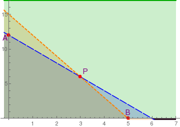
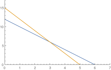
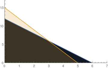
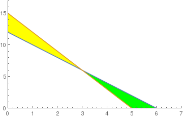
Note that we do not consider critical points outside the first quadrant because they have no biological meaning (population cannot be negative). If these two lines do not cross inside the first quadrant (\( x, y \ge 0 \) ), then there are only three equilibria on its boundary. In this case, the two species cannot coexist in peaceful equilibrium, and at least one of them will die out. This case is referred to as the competitive exclusion principle, Gause's law of competitive exclusion, or just Gause's law because it was originally formulated by Georgii Gause in 1934 on the basis of experimental evidence. It states that two species competing for the same resources cannot coexist if other ecological factors are constant. For instance, a competition in the 20th century between the USA and USSR resulted in the inevitable defeat of the latter.
Now we analyze stability of the given model using a linearization technique. We consider each equilibrium solution separately based on the properties of the corresponding Jacobian matrix:
\[
J(x,y) = \begin{bmatrix} r_1 -2a_1 x - b_1 y & -b_1 x \\ -b_2 y & r_2 - 2a_2 y - b_2 x \end{bmatrix} .
\]
The origin (0,0) is unstable node because its Jacobian
The point P is asymptotically stable. All other critical points are unstable. In terms of the ecology, this means that the interspecific competition is not too strong the two populations can coexist stably, but at lower populations than their respective carrying capacities. Thus, although the species may coexist, the price that they pay for competing with each other is that they do not reach the population density that they would have achieved (i.e. their carrying capacity) with the other species absent.
The critical point P is a saddle point (unstable). Points A and B on the boundary are asymptotically stable nodes. Therefore, in this case one of the populations extincts. This means that interspecific competition is aggressive and ultimately one population wins, while the other is driven to extinction. The winner depends upon which has the starting advantage.
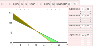
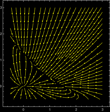
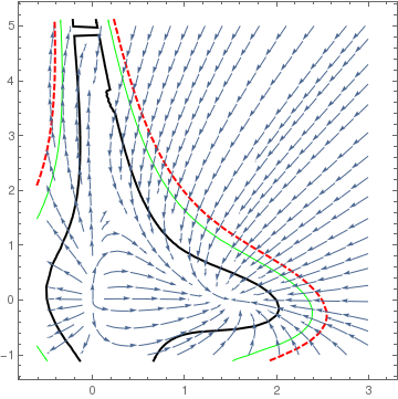
Example: Consider the following model that describes the competition between two species:
Since the eigenvalues of J(O) 19 and 13, the origin is an unstable node. Both points A and B are unstable saddle points because the their Jacobian matrices has one positive eigenvalue and one negative eigenvalue. The eigenvalues of matrix J(P) are
j[x_, y_] = {{19 - 6*x - y, -x}, {-y, 13 - x - 4*y}}
Eigenvalues[j[5,4]]
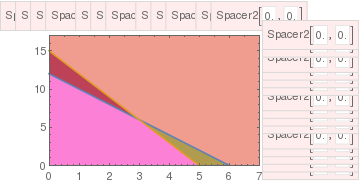
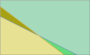
Obviously, the origin is unstable node because the linearized matrix has two positive eigenvalues. The eigenvalues of the Jacobian matrix at other critical points are
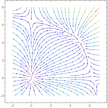
Since eigenvalues at points A and B are all negative, these points are asymptotically stable nodes. On the other hand, point P is a saddle point, so it is unstable.
■
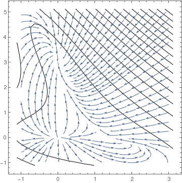
Example: Consider a
model that describes the competition between two species as
{{x -> 0, y -> 3}, {x -> 3/2, y -> 0}, {x -> 0, y -> 0}}
So this system has only three stationary points, and all of them are on the boundary. This means that one of populations will extinguish eventually.
According to given numerical values, we have
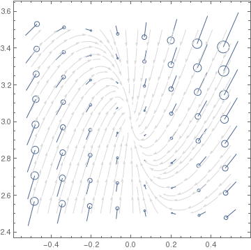
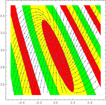
Therefore, the origin is unstable node, but point A(0,3) is an improper nodal sink (asymptotically stable). We cannot analyze point (3/2,0) using the linearization method because it is not isolated (one eigenvalue is zero). So we make another more closer look at its phase portrait.
Chi C-W, Hsu S-B, and Wu L-I., On the asymmetric May--Leonard model of three competing species, SIAM Journal on Applied Mathematics, 58, No 1, 1998, 211--226.
May R M and Leonard W J, Nonlinear aspects of competition between three species, SIAM Journal on Applied Mathematics, 29, No 2, 1975, 243--253. https://doi.org/10.1137/0129022
McGehee Richard and Armstrong Robert A., Some mathematical problems concerning the ecological principle of competitive exclusion, Journal of Differential Equations, 23, No 1, 1977, 30--52. doi: 10.1016/0022-0396(77)90135-8
Return to Mathematica page)
Return to the main page (APMA0340)
Return to the Part 1 Matrix Algebra
Return to the Part 2 Linear Systems of Ordinary Differential Equations
Return to the Part 3 Non-linear Systems of Ordinary Differential Equations
Return to the Part 4 Numerical Methods
Return to the Part 5 Fourier Series
Return to the Part 6 Partial Differential Equations
Return to the Part 7 Special Functions