Return to computing page for the first course APMA0330
Return to computing page for the second course APMA0340
Return to computing page for the fourth course APMA0360
Return to Mathematica tutorial for the first course APMA0330
Return to Mathematica tutorial for the second course APMA0340
Return to Mathematica tutorial for the fourth course APMA0360
Return to the main page for the first course APMA0330
Return to the main page for the second course APMA0340
Return to the main page for the fourth course APMA0360
Introduction to Linear Algebra with Mathematica
Glossary
Preface
This chapter is devoted to the most popular and extremely important in various applications of Fourier series and its generalizations. Joseph Fourier made in nineteen century a remarkable discovery of function's expansion defined on a prescribed finite interval into infinite series of trigonometric functions. Later on, it was recognized that Fourier series is just a particular case of more general topic (now called the harmonic analysis) of representing functions as a linear combination (generally speaking, with infinite terms) over an orthogonal set of eigenfunctions corresponding to some Sturm--Liouville problem. Fourier made a very important step in understanding series representation of functions because previously Taylor's series played the most dominated role. To some extend, the Fourier series (written in complex form) is a particular case of the Lauraunt series (which is a generalization of Taylor's series). However, Taylor's series are determined by infinitesimal behavior of a function at the center of expansion because its coefficients are defined through derivatives evaluated at one point. In contrast, Fourier coefficients depend on the behavior of a function on the whole interval.
Fourier series are strongly related to the Fourier integral transformations; however, due to space constraint, we present only one section in this topic and refer the reader to next chapter for some of its applications. Since Fourier coefficients are determined by integrals over a finite interval of interest, pointwise convergence is not very suitable to them. Therefore, we go in two directions. First we introduce the mean square convergence (also called in mathematics as 𝔏² or 𝔏2 convergence). Since pointwise convergence of Fourier series for piecewise functions leads to Gibbs phenomena, we suggest to use another type of convergence named after Italian mathematician Ernesto Cesàro. Its application to Fourier series is based on Fejér's theorem, named for Hungarian mathematician Lipót Fejér, who proved it in 1900 when he was 19 years old!
In the 19th century, Joseph Fourier wrote: “The study of Nature is the most productive source of mathematical discoveries. By offering a specific objective, it provides the advantage of excluding vague problems and unwieldy calculations. It is also a means to form the Mathematical Analysis, and isolate the most important aspects to know and to conserve. These fundamental elements are those which appear in all natural effects.”
A Fourier series is a particular case of a more general orthogonal expansion with respect to eigenfunctions of differential operators. In particular, its eigenfunctions \( \sin \frac{n\pi x}{\ell} \) and \( \cos \frac{n\pi x}{\ell} , \) where \( n=0,1,2,\ldots , \) are solutions of the following Sturm--Liouville problem:
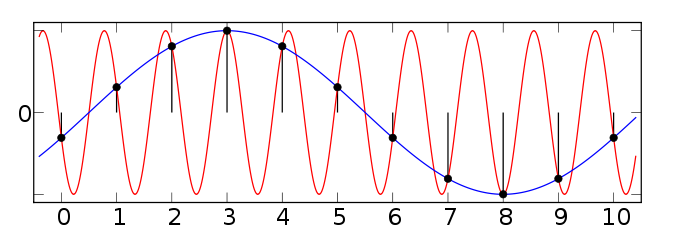
A Fourier series is a way to represent a function as the sum of simple sine waves. More formally, a Fourier series is a way to decompose a periodic function or periodic signal with a finite period \( 2\ell \) into an infinite sum of its projections onto an orthonormal basis that consists of trigonometric polynomials. Therefore, a Fourier series provides a periodic extension of a function initially defined on a finite interval of length \( 2\ell . \) They are named in honor of Jean-Baptiste Joseph Fourier (1768--1830), who used trigonometric series in representing solutions of partial differential equations, after preliminary investigations by Leonhard Euler (1707--1783), Jean le Rond d'Alembert (1717--1783), and Daniel Bernoulli (1700--1782).
Biography of Joseph Fourier
A Fourier series is a way of representing a periodic function as a (possibly infinite) sum of sine and cosine functions. It is actually a particular case of Taylor series, which represents functions as possibly infinite sums of monomial terms, when a variable belongs to the unit circle. For functions that are not periodic and defined on a finite interval, its Fourier series provides a periodic expansion from this interval.
Since the harmonic differential equation \( y'' + \lambda \,y =0 \) has periodic solutions, subject that λ is a positive number, it is convenient to represent its solution in complex form:
One can try to see other graphs by changing the input numbers. All the measurements are now on the circle in two dimensions. We call these “vectors”. Summing the vectors together give the final “power” of the frequency. This occurs when all the vectors line up and point in the same direction, creating high values that represent the “power” of the frequency.
Fourier series have a tremendous number of applications, of which we mention speech recognition and its applications in smart-phone communications due to its relevance today. Andrew Ng has long predicted that as speech recognition goes from 95% accurate to 99% accurate, it will become a primary way that we interact with computers. Contemporary smart phones constantly monitor sounds from the microphone, and when the owner says "hey Siri" or "ok google" followed by a question, it will respond to the owner. It only recognizes the owner's voice and not someone else’s so it uses sampling and comparison (with the Fourier series) to make sure your voice matches up with the samples it obtained when you first “trained” it.
The sounds we hear come from vibrations in air pressure. Humans do not hear all sounds: for example, we cannot hear the sound a dog whistle makes, but dogs can hear that sound. Marine animals can often hear sounds in a much higher frequency range than humans. What sound vibrations we can hear depends on the frequency and intensity of the air oscillations and one's individual hearing sensitivity. Frequency is the rate of repetition of a regular event. The number of cycles of a wave per second is expressed in units of hertz (Hz), in honor of the German physicist Heinrich Rudolf Hertz (1857--1894), who was the first to conclusively prove the existence of electromagnetic waves. Intensity is the average amount of sound power (sound energy per unit time) transmitted through a unit area in a specified direction; therefore, the unit of intensity is measured in watts per square meter. It is important to note that the sound intensity that scientists measure is not the same as loudness. Loudness describes how people perceive sound. Humans can hear sounds at frequencies from about 20 Hz to 20,000 Hz (or 20 kHz), though we hear sounds best at around 3,000 to 4,000 Hz, where human speech is centered. Scientists often specify sound intensity as a ratio, in decibels---the unit for intensity is the bel (dB), named in honor of the eminent British scientist Alexander Graham Bell (1847--1922), the inventor of the telephone---which is defined as 10 times the logarithm of the ratio of the intensity of a sound wave to a reference intensity.
When we detect sounds, or noise, our body is changing the energy in sound waves into nerve impulses which the brain then interprets. Such transmission occurs in human ears where sound waves cause the eardrum to vibrate. The vibrations pass through 3 connected bones in the middle ear, which causes fluid motion in the inner ear. Moving fluid bends thousands of delicate hair-like cells which convert the vibrations into nerve impulses that are carried to the brain by the auditory nerve; however, how the brain converts these electrical signals into what we ``hear'' is still unknown.
Sounds consist of vibrations in the air caused by its compression and decompression. Air is a gas containing atoms or molecules that can move freely in an arbitrary direction. The average velocity of air molecules at room temperature, under normal conditions, is around 450--500 meters per second. The mean free paths of air molecules before they collide with other air molecules is about 6 × 10⁻⁸ meters. So air consists of a large number of molecules in close proximity that collide with each other on average 1010 times per second, which is perceived as air pressure. When an object vibrates, it causes waves of increased and decreased pressure in the air that travel at about 340 meters per second.
The signals we use in the real world, such as our voices, are called
"analog" signals. To process these signals in computers, we need to
convert the signals to "digital" form. While an analog signal is
continuous in both time and amplitude, a digital signal is
discrete. To convert a continuous signal in time into a discrete one,
a process, called sampling. When the continuous analog signal
is sampled at a frequency f, the resulting discrete signal has
more frequency components than the analog signal did.
The periodic audio signals are known as (music) tones. A simple tone, or pure tone, has a sinusoidal waveform of amplitude a > 0, frequency ω0 > 0, and phase angle φ: \( x(t) = a\,\cos \left( \omega_0 t + \varphi \right) . \) The frequency ω0 has units of radians/second = 1/seconds, with t in seconds, and phase angle φ is in radians. An alternative is to express the frequency in units of Hertz, abbreviated Hz, given by f0 = ω0/(2π). The perceived loudness of a pure tone is proportional to a0.6. The pitch of a pure tone is logarithmically related to the frequency.
Sound is recorded through regular samples. These samples are
taken at a specified rate, named the
The information beyond 4 kHz is eliminated in the case of telephone
bandwidth speech. Even though the sampling frequency seems to be fine
for sounds like a and aa, it severely affects other sounds like s and
sh. However, information up to 4 kHz bandwidth seem to be sufficient
for intelligible speech. If the sampling frequency is further
decreased from 8 kHz, then intelligibility of speech degrades
significantly. Hence 8 kHz was chosen as the sampling frequency for
telephone communication. The speech signal sampled at 8 kHz is
termed as
Another important parameter of digitization is the process of quantization that consists of assigning a numerical value to each sample according to its amplitude. These numerical values are attributed according to a bit scale. A quantization of 8 bits will assign amplitude values along a scale of 28 = 256 states around 0 (zero). Most recording systems use a 216 = 65536 bit system. Quantization can be seen as a rounding process. A high bit quantization will produce values close to reality, i. e., values rounded to a high number of significant digits, whereas a low bit quantization will produce values far from reality, i.e., values rounded to a low number of significant digits. Low quantization can lead to impaired quality of the signal.
Sampling is a process of converting a signal (for example, a function of continuous time and/or space) into a numeric sequence (a function of discrete time and/or space). An analog-to-digital converter (ADC) can be modeled as two processes: sampling and quantization. Sampling converts a time-varying voltage signal into a discrete-time signal, a sequence of real numbers. Quantization replaces each real number with an approximation from a finite set of discrete values.
Fourier series applications are based on the fundamental sampling theorem that establishes a bridge between continuous-time signals (often called "analog signals") and discrete-time signals (often called "digital signals"). Strictly speaking, the theorem is only applied to a class of mathematical functions having a Fourier transform that is zero outside of a finite region of frequencies.
A sufficient sample-rate is therefore 2B samples/second, or anything larger. Equivalently, for a given sample rate fs, perfect reconstruction is deemed possible for a bandlimit B < fs/2. Therefore, the sampling theorem states that a signal can be exactly reproduced if it is sampled at a frequency greater than twice the maximum frequency in the signal.
In telephoning, the usable voice frequency band ranges from approximately 300 Hz to 3400 Hz.
The bandwidth allocated for a single voice-frequency transmission channel is usually 4 kHz, including guard bands, allowing a sampling rate of 8 kHz to be used as the basis of the pulse code modulation system used for the digital PSTN (Short-time Fourier Transform). This gives a 64 kbit/s digital signal known as DS0, which is subject to compression encoding using either μ-law (mu-law) PCM (North America and Japan) or A-law PCM (Europe and most of the rest of the world). Pulse-code modulation (PSM) ) is a method used to digitally represent sampled analog signals. According to the
Now we need to define the Fourier transform that decomposes a function of time (a signal) into the frequencies that make it up, in a way similar to how a musical chord can be expressed as the frequencies (or pitches) of its constituent notes. The Fourier transform of the function f is traditionally denoted by adding a circumflex:
- Peters, Terry M. editor, The Fourier Transform in Biomedical Engineering, Boston, MA : Birkhäuser, 1998.
- Serov, V., Fourier Series, Fourier Transform and Their Applications to Mathematical Physics, Springer International Publishing, 2017.
- Zaanen, A.C., Continuity, Integration and Fourier Theory, Springer Berlin Heidelberg, 1989.