Preface


This section presents solutions to the Laplace and Helmholtz equations with mixed boundary conditions in rectangular coordinates.

Return to computing page for the first course APMA0330
Return to computing page for the second course APMA0340
Return to Mathematica tutorial for the first course APMA0330
Return to Mathematica tutorial for the second course APMA0340
Return to the main page for the first course APMA0330
Return to the main page for the second course APMA0340
Return to Part VI of the course APMA0340
Introduction to Linear Algebra with Mathematica

Mixed Problems for Laplace and Helmholtz Equations


In this section, we consider boundary value problems for Laplace's and Helmholtz equations subject to the boundary condition of the third. This is a type of boundary condition that involve both the functions and its normal derivative in the boundary conditions:

\[ \left( a({\bf x})\,u({\bf x}) + b({\bf x})\,\frac{\partial u}{\partial {\bf n}} \right)_{\partial\Omega} \equiv \left( a({\bf x})\,u({\bf x}) + b({\bf x})\,\nabla u({\bf x}) \cdot {\bf n}({\bf x}) \right)_{\partial\Omega} = f({\bf x}), \qquad {\bf x} \in \partial\Omega , \]
where a and b are nonzero functions or constants, not simultaneously zero. The third type boundary conditions are variously designated, but frequently are called Robin's boundary conditions, which is mistakenly associated with the French mathematical analyst Victor Gustave Robin (1855--1897) from the Sorbonne in Paris. Actually, Robin never used this boundary condition as it follows from the historical research article:
Karl Gustafson and Takehisa Abe. The third boundary condition—was it robin’s? The Mathematical Intelligencer, March 1998, Volume 20, Issue 1, pp. 63--71.

Suppose we want to find the steady-state temperature u(x,y) in a rectangular plate with two insulated boundaries. When no heat escapes from the lateral faces of the plate, we solve Laplace's equation

\[ \frac{\partial^2 u }{\partial x^2} + \frac{\partial^2 u }{\partial y^2} =0 , \qquad 0 < x < a, \quad 0 < y < b , \] subject to mixed boundary conditions
\[ \left. \frac{\partial u }{\partial x} \right\vert_{x=0} =0 , \qquad \left. \frac{\partial u }{\partial x} \right\vert_{x=a} =0 , \qquad 0 < y < b , \]
and
\[ u(x,0) = f_0 (x) , \qquad u(x,b) = f_b (x) , \qquad 0 < x < a. \]
We seek partial nontrivial (= not identically zero) solutions of Laplace's equation subject to homogeneous boundary conditions in variable x (\( u_x (0,y) =0 \mbox{ and } u_x (a,) =0 \) ) and represented as \( u(x,y) = X(x)\,Y(y) . \) Substituting u = X Y into Laplace's equation, we get
\[ X'' (x)\,Y(y) + X(x)\,Y'' (y) =0 \qquad\Longrightarrow \qquad \frac{X''}{X} = -\frac{Y''}{Y} = - \lambda , \]
where λ is a constant. From the homogeneous boundary conditions,
\[ \left. \frac{\partial u }{\partial x} \right\vert_{x=0} = X' (0)\,Y(y) =0 \qquad\mbox{and}\qquad \left. \frac{\partial u }{\partial x} \right\vert_{x=a} = X'(a)\,Y(y) =0 , \]
we derive
\[ X' (0) =0, \qquad X' (a) =0 . \]
Therefore, we have the Sturm--Liouville problem for variable X:
\[ X'' + \lambda\,X =0, \qquad X' (0) =0, \quad X' (a) =0 . \]
The above problem has a sequence of nonegative eigenvalues and corresponding eigenfunctions:
\[ \lambda_n = \left( \frac{n\pi}{a} \right)^n , \qquad X_n (x) = \cos \frac{n\pi x}{a} , \qquad n=0,1,2,\ldots . \]
For Y, we have a similar differential equation
\[ Y'' - \lambda_n Y =0 \]
that has the general solution
\[ Y_n (y) = a_n \cosh \frac{n\pi y}{a} + b_n \sinh \frac{n\pi y}{a} , \qquad n=1,2,\ldots , \]
when \( n \ne 0 , \) and
\[ Y_0 (y) = a_0 + b_0 y , \]
when n = 0. Adding products of all partial solutions, we represent the required solution in the form of infinite series:
\[ u(x,y) = a_0 + b_0 y + \sum_{n\ge 1} \left[ a_n \cosh \frac{n\pi y}{a} + b_n \sinh \frac{n\pi y}{a} \right] \cos \frac{n\pi x}{a} . \]
To satisfy boundary conditions in y, we have
\begin{eqnarray*} u(x,0) &=& f_0 (x) = a_0 + \sum_{n\ge 1} a_n \cos \frac{n\pi x}{a} , \\ u(x,b) &=& f_a (x) = a_0 + b_0 b + \sum_{n\ge 1} \left[ a_n \cosh \frac{n\pi b}{a} + b_n \sinh \frac{n\pi b}{a} \right] \cos \frac{n\pi x}{a} . \end{eqnarray*}
Both equations are just cosine Fourier series for two input functions. So we easily find values of a's:
\begin{eqnarray*} a_0 &=& \frac{1}{a} \int_0^{a} f_0 (x)\, {\text d}x , \\ a_n &=& \frac{2}{a} \int_0^{a} f_0 (x)\, \cos \frac{n\pi x}{a}\, {\text d}x , \qquad n=1,2,3,\ldots . \end{eqnarray*}
Determination of other coefficients requires a little bit more work:
\begin{eqnarray*} b_0 &=& \frac{1}{ab} \int_0^{a} f_b (x)\, {\text d}x - \frac{a_0}{b} , \\ b_n &=& \frac{2}{a\,\sinh \frac{n\pi b}{a}} \, \int_0^{a} f_b (x)\, \cos \frac{n\pi x}{a}\, {\text d}x - a_n \mbox{coth} \frac{n\pi b}{a} , \qquad n=1,2,3,\ldots . \end{eqnarray*}

Laplace's equation is a second-order partial differential equation named after Pierre-Simon Laplace who, beginning in 1782, studied its properties while investigating the gravitational attraction of arbitrary bodies in space. However, the equation first appeared in 1752 in a paper by Euler on hydrodynamics. Laplace's equation is often written as:

\[ \Delta u ({\bf x}) =0 \qquad \mbox{in domain } {\bf x} \in \Omega \subset \mathbb{R}^n , \]
where \( \Delta = \nabla^2 \) is the Laplace operator or Laplacian. Another very important version of the above equation is so called the Helmholtz equation
\[ \Delta u ({\bf x}) + k^2 u =0 \qquad \mbox{in domain } {\bf x} \in \Omega \subset \mathbb{R}^n , \]
named for the German physician and physicist Hermann von Helmholtz (1821--1894). A nonhomogeneous version of the Laplace equation
\[ \Delta u ({\bf x}) = f({\bf x}) \qquad \mbox{in domain } \Omega \subset \mathbb{R}^n , \]
where f is a given smooth function, is called the Poisson's equation. The equation is named after the French mathematician, geometer, and physicist Siméon Denis Poisson (1781--1840). In two dimensions, the Laplace equation in rectangular coordinates becomes
\[ \frac{\partial^2 u}{\partial x^2} + \frac{\partial^2 u}{\partial y^2} =0 \qquad\mbox{or for short} \qquad u_{xx} + u_{yy} =0 . \]
Correspondingly, in three dimensions, the Poisson's equation is
\[ u_{xx} + u_{yy} + u_{zz} = f(x,y,z) , \]
where f is a given smooth function. The Laplacian occurs in differential equations that describe many physical phenomena, such as electric and gravitational potentials, the diffusion equation for heat and fluid flow, wave propagation, and quantum mechanics. The Laplacian represents the flux density of the gradient flow of a function. For instance, the net rate at which a chemical dissolved in a fluid moves toward or away from some point is proportional to the Laplacian of the chemical concentration at that point.

Since there is no time dependence in the Laplace's equation or Poisson's equation, there is no initial conditions to be satisfied by their solutions. However, there should be certain boundary conditions on the boundary curve or surface \( \partial\Omega \) of the region Ω in which the differential equation is to be solved. Typically, there are known three types of boundary conditions.

The problem of finding a solution of Laplace's equation that takes on given boundary values is known as a Dirichlet problem. On the other hand, if the values of the normal derivative are prescribed on the boundary, the problem is said to be a Neumann problem. Physically, it is plausible to expect that three types of boundary conditions will be sufficient to determine the solution completely. Indeed, it is possible to establish the existence and uniqueness of the solution of Laplace's (and Poisson's) equation under the first and third type boundary conditions, provided that the boundary \( \partial\Omega \) of the domain Ω is smooth (have no corner or edge). However, we avoid explicit statements and their proofs because the material is beyond the scope of the tutorial. Instead, we concentrate our attention on some typical problems that could be solved by means of separation of variables.

Neumann Problem for a Rectangle

The general interior Neumann problem for Laplace's equation for rectangular domain \( [0,a] \times [0,b] , \) in Cartesian coordinates can be formulated as follows. Find solution of Laplace's equation
\[ \Delta u \equiv u_{xx} + u_{yy} =0 , \qquad 0 < x < a, \quad 0< y <b ; \]
subject to the boundary conditions of the second kind
\[ \left. \frac{\partial u}{\partial x} \right\vert_{x=0} = u_x (0,y) = g_0 (y) , \qquad \left. \frac{\partial u}{\partial x} \right\vert_{x=a} = u_x (a,y) = g_a (y) , \qquad 0 < y < b, \]
and
\[ \left. \frac{\partial u}{\partial y} \right\vert_{y=0} = u_y (x,0) = f_0 (x) , \qquad \left. \frac{\partial u}{\partial y} \right\vert_{y=b} = u_y (x,b) = f_b (x) , \qquad 0 < x < a ; \]
where f0, fb, g0, and ga are give functions. Here we use the shortcut notation ux and uy for partial derivatives with respect to x and y, respectively.

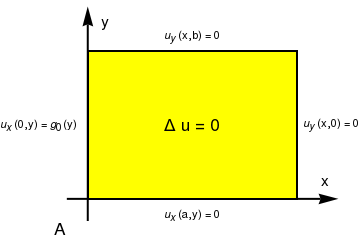
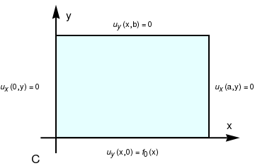
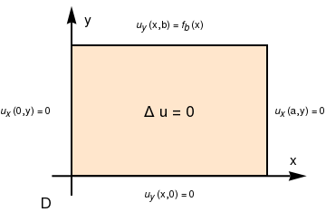
Using superposition principle, we can break the given Neumann problems into four similar problems when flux source comes only from one side of the rectangle, and other three sides are isolated. Hence, we can represent the solution as the sum of four functions

\[ u(x,y) = u_A (x,y) + u_B (x,y) + u_C (x,y) + u_D (x,y) , \]
each of them is a solution of Laplace's equation with insulated three sides. Therefore, we get four Neumann problems. (Be aware that you browser may not display the codes properly.) Note that problems A and B could be united into one, as well as problems C and D.
rectangle = Graphics[{EdgeForm[Thick], Yellow, Rectangle[{0, 0}, {3, 2}]}];
aA = Graphics[Text[Style["A", FontSize -> 16], {-0.4, -0.4}]];
a0 = Graphics[ Text[Style[ "\!\(\*SubscriptBox[\(u\), \(x\)]\)(a,y) = 0"], {1.5, -0.2}]];
a1 = Graphics[ Text[Style["\!\(\*SubscriptBox[\(u\), \(y\)]\)(x,0) = 0"], {3.5, 1.0}]];
a2 = Graphics[ Text[Style["\!\(\*SubscriptBox[\(u\), \(y\)]\)(x,b) = 0"], {1.5, 2.2}]];
ax = {Arrowheads[Large], Arrow[{{-0.3, 0}, {3.6, 0}}]};
ax1 = Graphics[{Thick, Black, ax}];
ay = {Arrowheads[Large], Arrow[{{0, -0.3}, {0, 2.6}}]};
ay1 = Graphics[{Thick, Black, ay}];
txt1 = Graphics[Text[Style["x", FontSize -> 14], {3.4, 0.25}]];
txt2 = Graphics[Text[Style["y", FontSize -> 14], {0.25, 2.4}]];
left = Graphics[ Text[Style[ "\!\(\*SubscriptBox[\(u\), \(x\)]\)(0,y) = \ \!\(\*SubscriptBox[\(g\), \(0\)]\)(y)"], {-0.7, 1}]];
delta = Graphics[ Text[Style["\[CapitalDelta] u = 0", FontSize -> 16], {1.5, 1.0}]];
Show[ax1, ay1, rectangle, txt1, txt2, delta, left, a0, a1, a2, aA, AspectRatio -> 3/4]
rectangleB = Graphics[{EdgeForm[Thick], Pink, Rectangle[{0, 0}, {3, 2}]}];
right = Graphics[ Text[Style[ "\!\(\*SubscriptBox[\(u\), \(x\)]\)(a,y) = \ \!\(\*SubscriptBox[\(g\), \(a\)]\)(y)"], {3.8, 1}]];
a0 = Graphics[ Text[Style["\!\(\*SubscriptBox[\(u\), \(x\)]\)(0,y) = 0"], {-0.7, 1.0}]];
a1 = Graphics[ Text[Style[ "\!\(\*SubscriptBox[\(u\), \(y\)]\)(x,0) = 0"], {1.5, -0.3}]];
a2 = Graphics[ Text[Style["\!\(\*SubscriptBox[\(u\), \(y\)]\)(x,b) = 0"], {1.5, 2.2}]];
aB = Graphics[Text[Style["B", FontSize -> 16], {-0.4, -0.4}]];
Show[rectangleB, right, txt1, txt2, ax1, ay1, a0, a1, a2, aB]
rectangleC = Graphics[{EdgeForm[Thick], LightCyan, Rectangle[{0, 0}, {3, 2}]}];
down = Graphics[ Text[Style[ "\!\(\*SubscriptBox[\(u\), \(y\)]\)(x,0) = \ \!\(\*SubscriptBox[\(f\), \(0\)]\)(x)"], {1.5, -0.3}]];
a0 = Graphics[ Text[Style["\!\(\*SubscriptBox[\(u\), \(x\)]\)(0,y) = 0"], {-0.7, 1.0}]];
a1 = Graphics[ Text[Style["\!\(\*SubscriptBox[\(u\), \(x\)]\)(a,y) = 0"], {3.5, 1.0}]];
a2 = Graphics[ Text[Style["\!\(\*SubscriptBox[\(u\), \(y\)]\)(x,b) = 0"], {1.5, 2.2}]];
aC = Graphics[Text[Style["C", FontSize -> 16], {-0.4, -0.4}]];
Show[rectangleC, down, txt1, txt2, ax1, ay1, a0, a1, a2, aC]
rectangleD = Graphics[{EdgeForm[Thick], LightOrange, Rectangle[{0, 0}, {3, 2}]}];
top = Graphics[ Text[Style[ "\!\(\*SubscriptBox[\(u\), \(y\)]\)(x,b) = \ \!\(\*SubscriptBox[\(f\), \(b\)]\)(x)"], {1.5, 2.3}]];
a0 = Graphics[ Text[Style["\!\(\*SubscriptBox[\(u\), \(x\)]\)(0,y) = 0"], {-0.7, 1.0}]];
a1 = Graphics[ Text[Style["\!\(\*SubscriptBox[\(u\), \(x\)]\)(a,y) = 0"], {3.5, 1.0}]];
a2 = Graphics[ Text[Style[ "\!\(\*SubscriptBox[\(u\), \(y\)]\)(x,0) = 0"], {1.5, -0.3}]];
aD = Graphics[Text[Style["D", FontSize -> 16], {-0.4, -0.4}]];
Show[rectangleD, top, txt1, txt2, ax1, ay1, a0, a1, a2, aD, delta]

Problem A consists of the partial differential equation \( \Delta u =0 \) in the rectangle \( (0,a) \times (0,b) \) subject to the boundary conditions:

\[ \left. \frac{\partial u}{\partial x} \right\vert_{x=0} = u_x (0,y) = g_0 (y) , \qquad \left. \frac{\partial u}{\partial x} \right\vert_{x=a} = u_x (a,y) = 0, \qquad 0 < y < b;\qquad \left. \frac{\partial u}{\partial y} \right\vert_{y=0} = u_y (x,0) = 0 , \qquad \left. \frac{\partial u}{\partial y} \right\vert_{y=b} = u_y (x,b) = 0 . \]
To solve problem A, we proceed in exactly the same as in the previous problem: set \( u(x,y) = X(x)\,Y(y) \) and substitute into the Laplace equation and homogeneous boundary conditions in y. This give the familiar Sturm--Liouville problem for Y:
\[ Y'' + \lambda\,Y =0 , \qquad Y'(0) =0, \quad Y'(b) =0. \]
Its solution is well-known:
\[ \lambda_n = \left( \frac{n\pi}{b} \right)^2 , \qquad Y_n (y) = \cos \frac{n\pi y}{b} , \qquad n=0,1,2,\ldots . \]
Note that zero is an eigenvalue to which corresponds a constant eigenfunction. For X, we get the following differential equation:
\[ X'' (x) - \left( \frac{n\pi}{b} \right)^2 X(x) =0 , \]
which has the general solution
\[ X_n (x) = c_{1n} \cosh \frac{n\pi x}{b} + c_{2n} \sinh \frac{n\pi x}{b} . \]
The solution of the given Neumann problem A for Laplace's equation is assumed to be represented as the sum of all partial nontrivial solutions:
\[ u(x,y) = C+\sum_{n\ge 1} X_n (x)\, Y_n (y) , \]
where C is an arbitrary constant. Since each term in the above sum satisfies the homogeneous boundary conditions \( u_y (x,0) = u_y (x,b) =0 , \) we know that the sum has the same property (subject to uniform convergence, which is assumed). To satisfy the boundary conditions in variable x, we have to consider two equations
\[ u_x (0,y) = \sum_{n\ge 1} X'_n (0)\, Y_n (y) = g_0 (y) \qquad\mbox{and} \qquad u_x (a,y) = \sum_{n\ge 1} X'_n (a)\, Y_n (y) = 0 . \]

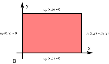
Problem B consists of the partial differential equation \( \Delta u =0 \) in the rectangle \( (0,a) \times (0,b) \) subject to the boundary conditions:

\[ \left. \frac{\partial u}{\partial x} \right\vert_{x=0} = u_x (0,y) = 0 , \qquad \left. \frac{\partial u}{\partial x} \right\vert_{x=a} = u_x (a,y) = g_a (y) \qquad 0 < y < b;\qquad \left. \frac{\partial u}{\partial y} \right\vert_{y=0} = u_y (x,0) = 0 , \qquad \left. \frac{\partial u}{\partial y} \right\vert_{y=b} = u_y (x,b) = 0 . \]
Note that it has homogeneous boundary conditions in variable y. To solve problem B, we proceed in exactly the same as in the previous problem: set \( u(x,y) = X(x)\,Y(y) \) and substitute into the Laplace equation and homogeneous boundary conditions in y. This give the familiar Sturm--Liouville problem for Y:
\[ Y'' + \lambda\,Y =0 , \qquad Y'(0) =0, \quad Y'(b) =0. \]
Its solution is well-known:
\[ \lambda_n = \left( \frac{n\pi}{b} \right)^2 , \qquad Y_n (y) = \cos \frac{n\pi y}{b} , \qquad n=0,1,2,\ldots . \]
Note that zero is an eigenvalue to which corresponds a constant eigenfunction. For X, we get the following differential equation:
\[ X'' (x) - \left( \frac{n\pi}{b} \right)^2 X(x) =0 , \]
which has the general solution
\[ X_n (x) = c_{1n} \cosh \frac{n\pi x}{b} + c_{2n} \sinh \frac{n\pi x}{b} . \]
The solution of the given Neumann problem B for Laplace's equation is assumed to be represented as the sum of all partial nontrivial solutions:
\[ u(x,y) = C+\sum_{n\ge 1} X_n (x)\, Y_n (y) , \]
where C is an arbitrary constant. Since each term in the above sum satisfies the homogeneous boundary conditions \( u_y (x,0) = u_y (x,b) =0 , \) we know that the sum has the same property (subject to uniform convergence, which is assumed). To satisfy the boundary conditions in variable x, we have to consider two equations
\[ u_x (0,y) = \sum_{n\ge 1} X'_n (0)\, Y_n (y) =0 \qquad\mbox{and} \qquad u_x (a,y) = \sum_{n\ge 1} X'_n (a)\, Y_n (y) = g_a (y) . \]
Therefore, if we set \( X'_n (0) =0 , \) which is equivalent to \( c_{2n} =0, \) it will guarantee that the first boundary condition holds. With this in hand, we obtain the general solution:
\[ u(x,y) = C+\sum_{n\ge 1} X_n (x)\, Y_n (y) = C+\sum_{n\ge 1} A_n \cosh \frac{n\pi x}{b} \, \cos \frac{n\pi y}{b} , \]
where coefficients An should be chosen so that the identity
\[ \left. \frac{\partial u}{\partial x} \right\vert_{x=a} = \sum_{n\ge 1} X'_n (a)\, Y_n (y) = \sum_{n\ge 1} A_n \,\frac{n\pi }{b} \, \sinh \frac{n\pi a}{b} \, \cos \frac{n\pi y}{b} = g_a (y) . \]
is valid. However, this is just Fourier cosine series for function g, and its coefficients follow from Euler's formulas:
\[ A_n \,\frac{n\pi }{b} \, \sinh \frac{n\pi a}{b} = \frac{2}{b} \int_0^b g_a (y)\, \cos \frac{n\pi y}{b} \,{\text d}y \qquad \Longrightarrow \qquad A_n = \dfrac{2}{n\pi \, \sinh \frac{n\pi a}{b}} \, \int_0^b g_a (y)\, \sin \frac{n\pi y}{b} \,{\text d}y , \qquad n=1,2,3,\ldots . \]
Since the constant term in cosine Fourier series is absent, the above expansion is valid only when
\[ \int_0^b g_a (y)\,{\text d}y =0. \]
In this case, the Neumann problem has a solution up to arbitrary constant, so it is not unique. ■


Return to Mathematica page
Return to the main page (APMA0340)
Return to the Part 1 Matrix Algebra
Return to the Part 2 Linear Systems of Ordinary Differential Equations
Return to the Part 3 Non-linear Systems of Ordinary Differential Equations
Return to the Part 4 Numerical Methods
Return to the Part 5 Fourier Series
Return to the Part 6 Partial Differential Equations
Return to the Part 7 Special Functions