Preface
This section gives an example of the chaotic dynamic system known as the Rössler attractor. It is a system of three non-linear ordinary differential equations originally studied by Otto Rössler (born 1940) in the 1970's. These differential equations define a continuous-time dynamical system that exhibits chaotic dynamics associated with the fractal properties of the attractor.
Return to computing page for the second course APMA0340
Return to Mathematica tutorial for the first course APMA0330
Return to Mathematica tutorial for the second course APMA0340
Return to the main page for the first course APMA0330
Return to the main page for the second course APMA0340
Return to Part I of the course APMA0340
Introduction to Linear Algebra with Mathematica
Glossary
The Rössler attractor is the attractor for the Rössler system, a system of three non-linear ordinary differential equations originally studied by the German biochemist Otto Eberhard Rössler (born 20 May 1940).
- Rössler, O. E. (1976), "An equation for continuous chaos", Physics Letters A, 57 (5): 397--398.
- Rössler, O. E. (1979), "An Equation for Hyperchaos", Physics Letters, 71A (2,3): 155--157.
- Rössler, Otto E. (1976). "Chaotic behavior in simple reaction system". Zeitschrift für Naturforschung A. 31: 259–264.
- Letellier, C.; V. Messager (2010). "Influences on Otto E. Rössler’s earliest paper on chaos". International Journal of Bifurcation & Chaos. 20 (11): 3585–3616.
Rössler and his wife Reimara have been involved with a long-running series of disputes with their employer, the University of Tübingen, which they accuse of discrimination and of violations of academic freedom. In 1988, Reimara Rössler, a professor of medicine, was transferred to a different department within the university; in protest, she began working from home. The state of Baden-Württemberg sued her for failure to perform her assigned duties, as a result of which by 1996 she lost her job and was forced to give up a second home to refund her back pay. Meanwhile, in 1993 and 1994, Otto Rössler had been assigned to teach an introductory chemistry course according to the prescribed curriculum for medical students, but insisted instead on teaching his own material. After he was replaced in the course by another lecturer, he continued trying to give the lectures himself, and was removed by police several times. Because of these incidents, in 1995 a state official tried to force Rössler to undergo psychological tests, but after international protests by many academics this plan was dropped. Rössler continued protesting against his and his wife's treatment by the university and in August 2001 he was caught defacing the university auditorium with spray paint in an attempt to draw attention to his protests.
In 1976, Rössler considered the system of ordinary differential equations
These Rössler equations are simpler than those Lorenz used since only one nonlinear term appears (the product xz in the third equation). Otto Rössler solved these equations on a computer. When he made a phase space diagram with the variables, he obtained what has become known as the “Rössler attractor.”
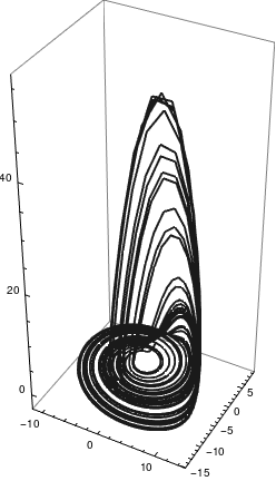
Example 1: Consider the Rössler system of equations with parameter values 𝑎 = 0.32, b = 0.3, and c = 5.8. We plot its solution using the following code:
sol1 = NDSolve[{x'[t] == -(y[t] + z[t]), y'[t] == x[t] + a* y[t],
z'[t] == b + x[t] z[t] - c* z[t], x[0] == 1, y[0] == 2, z[0] == 3}, {x, y, z}, {t, 0, 200}]
ParametricPlot3D[Evaluate[{x[t], y[t], z[t]} /. sol1], {t, 0, 200}, WorkingPrecision -> 22, PlotRange -> All, PlotTheme -> "Monochrome"]
|
|
|
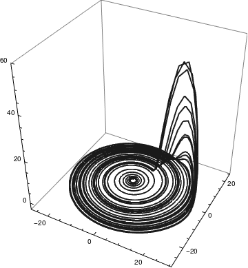
| Rössler attractor for 𝑎 = 0.32, b = 0.3, and c = 5.8 | Rössler attractor for 𝑎 = 0.1, b = 0.1, and c = 18 |

{{sol}, {pts}} =
Reap[NDSolve[{x'[t] == -(y[t] + z[t]), y'[t] == x[t] + a y[t],
z'[t] == b + x[t] z[t] - c z[t], x[0] == 1, y[0] == 2, z[0] == 3,
WhenEvent[z'[t] == 0, Sow[t]]}, {x, y, z}, {t, 0, 100}]];
z = z /. sol;
maxPts = Last /@ Partition[pts, 2];
Plot[z[t], {t, 0, 100}, PlotRange -> All, Epilog -> Point[{#, z[#]} & /@ maxPts]]

Plane Case
Setting z = 0, allows examination of the behavior on the x,y plane
which is a linear system of ODEs. The stability in the x,y plane can then be found by calculating the eigenvalues of the Jacobian \( \begin{bmatrix} 0& -1 \\ 1&a \end{bmatrix} , \) which are \( \left( a \pm \sqrt{a^2 -4} \right) /2 . \) From this, we can see that when 0 < a < 2, the eigenvalues are complex and both have a positive real component, making the origin unstable with an outwards spiral on the x,y plane. Now consider the z-plane behavior within the context of this range for a. So long as x is smaller than c, the c term will keep the orbit close to the x,y plane. As the orbit approaches x greater than c, the z-values begin to climb. As z climbs, though, the -z in the equation for \( \dot{x} \) stops the growth in x.
Fixed points
In order to find the fixed points, the three Rössler equations are set to zero and the (x,y,z) coordinates of each fixed point were determined by solving the resulting equations. This yields the general equations of each of the fixed point coordinates:
Topological description
The topology of the Rössler attractor was first described in terms of a paper-sheet model. Typically, the paper-sheet model can be divided in two stripes, one being a "normal band" and one being a Möbius band. These two bands thus define two different topological domains. In the 1990's, such a topological description led to the concept of a branched manifold, also called knot-holder or template. It can be shown that such a paper-sheet model encodes all topological properties of the unstable periodic orbits embedded within the attractor. The Rössler attractor is the most simple chaotic attractor from the topological point of view, that is, it is a simple stretched and folded ribbon.
Eigenvalues and eigenvectors
The stability of each of these fixed points can be analyzed by determining their respective eigenvalues and eigenvectors. Beginning with the Jacobian
These eigenveluess have several interesting implications. First, the two complex eigenvalues are responsible for the steady outward slide that occurs in the main disk of the attractor. The last negative eigenvalue is attracting along an axis that runs through the center of the manifold and accounts for the z motion that occurs within the attractor. This effect is roughly demonstrated with the figure below.
Poincaré map
The Poincaré map is constructed by plotting the value of the function every time it passes through a set plane in a specific direction. An example would be plotting the y,z value every time it passes through the x = 0 plane where x is changing from negative to positive, commonly done when studying the Lorenz attractor. In the case of the Rössler attractor, the x = 0 plane is uninteresting, as the map always crosses the x = 0 plane at z = 0 due to the nature of the Rössler equations. In the x = 0.1 plane for a = 0.1, b = 0.1, c = 14, the Poincaré map shows the upswing in z values as x increases, as is to be expected due to the upswing and twist section of the Rössler plot. The number of points in this specific Poincaré plot is infinite, but when a different c value is used, the number of points can vary. For example, with a c value of 4, there is only one point on the Poincaré map, because the function yields a periodic orbit of period one, or if the c value is set to 12.8, there would be six points corresponding to a period six orbit.
Variation of parameters
Rössler attractor's behavior is largely a factor of the values of its constant parameters a, b, and c. In general, varying each parameter has a comparable effect by causing the system to converge toward a periodic orbit, fixed point, or escape towards infinity, however the specific ranges and behaviors induced vary substantially for each parameter. Periodic orbits, or "unit cycles," of the Rössler system are defined by the number of loops around the central point that occur before the loops series begins to repeat itself.
Varying a
Here, b is fixed at 0.2, c is fixed at 5.7 and a changes. Numerical examination of the attractor's behavior over changing a suggests it has a disproportional influence over the attractor's behavior. The results of the analysis are:
- \( a \le 0: \) converges to the centrally located fixed point.
- a = 0.1: unit cycle of period 1.
- a = 0.2: standard parameter value selected by Rössler, chaotic.
- a = 0.3: chaotic attractor, significantly more Möbius strip-like (folding over itself).
- a = 0.35: similar to 0.3, but increasingly chaotic.
- a = 0.38: Similar to 0.35, but increasingly chaotic.
Varying b
Here, a is fixed at 0.2, c is fixed at 5.7 and b changes. As shown in the accompanying diagram, as b approaches 0 the attractor approaches infinity (note the upswing for very small values of b. Comparative to the other parameters, varying b generates a greater range when period-3 and period-6 orbits will occur. In contrast to a and c, higher values of b converge to period-1, not to a chaotic state.
Varying c
Here, a = b = 0.1 and c changes. The bifurcation diagram reveals that low values of c are periodic, but quickly become chaotic as c increases. This pattern repeats itself as c increases --- there are sections of periodicity interspersed with periods of chaos, and the trend is towards higher-period orbits as c increases. For example, the period one orbit only appears for values of c around 4 and is never found again in the bifurcation diagram. The same phenomenon is seen with period three; until c = 12, period three orbits can be found, but thereafter, they do not appear.
- c = 4, period-1 orbit.
- c = 6, period-2 orbit.
- c = 8.5, period-4 orbit.
- c = 8,7, period-8 orbit.
- c = 9,sparse chaotic attractor.
- c = 12, period-3 orbit.
- c = 12,6, period-6 orbit.
- c = 13, sparse chaotic attractor.
- c = 18, filled-in chaotic attractor.
Simulation
Because three simultaneous equations are involved, with one of them being nonlinear, simulating the Rössler equations is not a simple task unless you are an experienced researcher. Glen Kleinschmidt in Australia has an excellent website ( glensstuff.com ) that deals with a variety of interesting topics. One of the things he discusses is simulating the Rössler equations and generating the Rössler attractor using LTspice.
Rössler hyperchaotic equations
In 1979, Otto Rössler developed a set of four equations that described an autonomous “hyperchaotic” system. The word “hyperchaotic” means that the system of equations must be at least four-dimensional (four variables). In addition, there must be two or more positive Lyapunov coefficients and the sum of all the Lyapunov coefficients must be negative.
The hyperchaotic set of equations that Rössler devised was:
It is important to note that when simulating or constructing Chau’s circuit, we are working with an actual oscillator electronic circuit. However, when dealing with the Rössler attractor, what we are simulating is an analog computer circuit which solves the Rössler equations.
Return to Mathematica page
Return to the main page (APMA0340)
Return to the Part 1 Matrix Algebra
Return to the Part 2 Linear Systems of Ordinary Differential Equations
Return to the Part 3 Non-linear Systems of Ordinary Differential Equations
Return to the Part 4 Numerical Methods
Return to the Part 5 Fourier Series
Return to the Part 6 Partial Differential Equations
Return to the Part 7 Special Functions