Return to computing page for the first course APMA0330
Return to computing page for the second course APMA0340
Return to computing page for the fourth course APMA0360
Return to Mathematica tutorial for the first course APMA0330
Return to Mathematica tutorial for the second course APMA0340
Return to Mathematica tutorial for the fourth course APMA0360
Return to the main page for the first course APMA0330
Return to the main page for the second course APMA0340
Return to the main page for the fourth course APMA0360
Return to Part III of the course APMA0340
Introduction to Linear Algebra with Mathematica
Glossary
Preface
This section addresses an introduction to the fasinated topic that originated from the work of the American mathematician and meteorologist Edward Norton Lorenz (1917--2008). He discovered what is known now as the deterministic chaos in mathematics and physics. The deterministic nature of dynamic systems does not make them predictable (determined) in practice. Solutions of differential systems involving more than two nonlinear differential equations may be qualitatively different from the planar solutions since slight pertubation may leads to exponential deviation. The chaos was summarised by Edward Lorenz as: Chaos – when the present determines the future, but the approximate present does not approximately determine the future.
The history of Lorenz discovery can be found in James Gleick (born 1954) book Gleick, formerly a science writer for the New York Times, depicts the beginnings of Chaos theory, which draws on the seemingly random patterns that characterize many natural phenomena. It explains the thought processes and investigative techniques of Chaos scientists, illustrating concepts like Julia sets, Lorenz attractors, and the Mandelbrot Set with sketches, photographs, and wonderful descriptive prose. This highly readable international best-seller is must-reading for any Clausewitzian. (See Alan D. Beyerchen's essay on the connection with Clausewitz.) ISBN: 0143113453.
Lorenz equations
We will wrap up this series of examples with a look at the fascinating Lorenz attractor. The Lorenz system (the Lorenz equations, note it is not Lorentz) is a three-dimensional system of ordinary differential equations that depends on three real positive parameters. They were first studied by the professor of MIT Edward Norton Lorenz (1917--2008) in 1963. Edward N. Lorenz, a meteorologist who tried to predict the weather with computers by solving a system of ordinary differential equations (now bearing his name) for certain parameter values and initial conditions, but instead gave rise to the modern field of chaos theory. For some parameter values, numerically computed solutions of the equations oscillate, apparently forever, in the pseudo-random way we now call "chaotic". In addition, there are some parameter values for which we see "preturbulence", a phenomenon in which trajectories oscillate chaotically for long periods of time before finally settling down to stable stationary or stable periodic behaviour, others in which we see "intermittent chaos", where trajectories alternate between chaotic and apparently stable periodic behaviours, and yet others in which we see "noisy periodicity", where trajectories appear chaotic though they stay very close to a non-stable periodic orbit.
An important problem in meteorology and in other applications of fluid dynamics is modeling a layer of fluid such as the earth's atmosphere. (Lorenz's derivation (1963) was based on considering a two-dimensional fluid cell (or layer) that is warmed from below and cooled from above. If the vertical temperature difference ΔT is small, then there is a linear variation of temperature with altitude, but no significant motion of the fluid layer. However, if ΔT is large enough, then the warmer air rises, displacing the cooler air above it, and steady convective motion results. If the temperature difference increases further, then eventually the steady convective flow breaks up and a more complex and turbulent motion ensues. Edward Lorenz was led to the nonlinear autonomous dynamic system:
Edward Lorenz was born in West Hartford, Connecticut. He studied mathematics at both Dartmouth College in New Hampshire and Harvard University in Cambridge, Massachusetts. From 1942 until 1946, he served as a meteorologist for the United States Army Air Corps. After his return from World War II, he decided to study meteorology. Lorenz earned two degrees in the area from the Massachusetts Institute of Technology. Dr. Lorenz was a staff member of M.I.T.’s meteorology department from 1948 to 1955, when he became an assistant professor. He was promoted to professor in 1962 and served as head of the department from 1977 to 1981. During the 1950s, Lorenz became skeptical of the appropriateness of the linear statistical models in meteorology, as most atmospheric phenomena involved in weather forecasting are non-linear. His work on the topic culminated in the publication of his 1963 paper "Deterministic Nonperiodic Flow" in Journal of the Atmospheric Sciences, and with it, the foundation of chaos theory. He was awarded the Kyoto Prize for basic sciences, in the field of earth and planetary sciences, in 1991.
Dr. Lorenz is best known for the notion (in 1969) of the “butterfly effect,” the idea that a small disturbance like the flapping of a butterfly’s wings can induce enormous consequences. His chaos discovery was accidental. One day, Dr. Lorenz was running simulations of weather using a simple computer model. Another day, he wanted to repeat one of the simulations for a longer time, but instead of repeating the whole simulation, he started the second run in the middle, typing in numbers from the first run for the initial conditions. The computer program was the same, so the weather patterns of the second run should have exactly followed those of the first. Instead, the two weather trajectories quickly diverged on completely separate paths.
At first, he thought the computer was malfunctioning. Then he realized that he had not entered the initial conditions exactly. The computer stored numbers to an accuracy of six decimal places, like 0.506127, while, to save space, the printout of results shortened the numbers to three decimal places, 0.506. When typing in the new conditions, Dr. Lorenz had entered the rounded-off numbers, and even this small discrepancy, of less than 0.1 percent, completely changed the final result. Even though his model was vastly simplified, Dr. Lorenz realized that this meant perfect weather prediction was a fantasy. A perfect forecast would require not only a perfect model, but also perfect knowledge of wind, temperature, humidity and other conditions everywhere around the world at one moment of time. Even a small discrepancy could lead to completely different weather. In 1972, he gave a talk with a title that captured the essence of his ideas: “Predictability: Does the Flap of a Butterfly’s Wings in Brazil Set Off a Tornado in Texas?”
In his later years, Lorenz lived in Cambridge, Massachusetts. He was an avid outdoorsman, who enjoyed hiking, climbing, and cross-country skiing. He kept up with these pursuits until very late in his life, and managed to continue most of his regular activities until only a few weeks before his death. According to his daughter, Cheryl Lorenz, Lorenz had "finished a paper a week ago with a colleague." On April 16, 2008, Lorenz died at his home in Cambridge at the age of 90, having suffered from cancer.
The Lorenz equations are made up of three populations: x, y, and z, and three fixed coefficients: σ, ρ, and β. Remembering what we discussed previously, this system of equations has properties common to most other complex systems, such as lasers, dynamos, thermosyphons, brushless DC motors, electric circuits, and chemical reactions. First, it is non-linear in two places: the second equation has a xz term and the third equation has a xy term. It is made up of a very few simple components. The system is three-dimensional and deterministic. Although difficult to see until we plot the solution, the equation displays broken symmetry on multiple scales. Because the equation is autonomous (no t term in the right side of the equations), there is no feedback in this case.
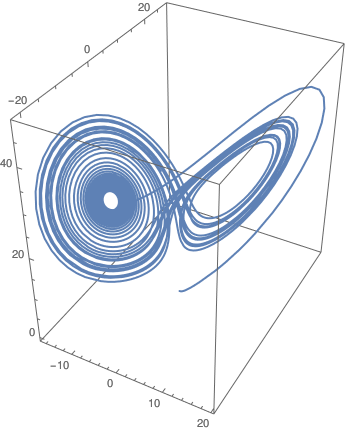
Because the three equations \eqref{EqLorenz.1} are so codependent, their trajectories orbit back and forth between two centers but never cross. Such properties (combined with the sensitivity to initial conditions) are what makes systems chaotic. This system’s behavior depends on the three constant values chosen for the coefficients. It has been shown that the Lorenz System exhibits complex behavior when the coefficients have the following specific values: \( \sigma = 10, \ \rho = 28 , \mbox{ and }\ \beta = 8/3. \) We now have everything we need to code up the ODE into Mathematica:
Example 1: We consider the Lorenz's equations under the following avlues of parameters:
|
\[Sigma] = 10;
solution = NDSolve[{x'[t] == \[Sigma] (y[t] - x[t]), y'[t] == 28 x[t] - y[t] - x[t] z[t], z'[t] == x[t] y[t] - 8/3 z[t], x[0] == z[0] == 0, y[0] == 2}, {x, y, z}, {t, 0, 35}] ParametricPlot3D[Evaluate[{x[t], y[t], z[t]} /. solution], {t, 0, 35}] |
|
| Lorenz attractor. | Mathematica code |
■
Example 2: We seek solutions of the Lorenz equations as power series
|
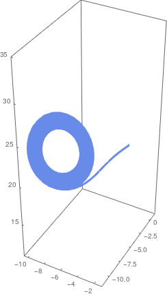
Here is Mathematica code for ploting Glukhovsky-Dolzhansky system:
\[Sigma] = 10; a = 0; r = 24; b = 8/3;
s = NDSolve[{x'[t] == -\[Sigma]*(x[t] - y[t]) - a*(y[t]*z[t]), y'[t] == r*x[t] - y[t] - x[t]*z[t], z'[t] == -b*z[t] + x[t]*y[t], x[0] == z[0] == 0, y[0] == 2}, {x, y, z}, {t, 0, 100}]; ParametricPlot3D[Evaluate[{x[t], y[t], z[t]} /. s], {t, 0, 70}, PlotTheme -> "Business"] |
|
| Solution of Glukhovsky-Dolzhansky system. | Mathematica code |
I is the moment of inertia of the wheel,
θ is the angle of the wheel,
\( \omega = \dot{\theta} \) is the angular velocity (increases counterclockwise, as does θ),
K is is the liquid’s leakage rate,
ν is the rotational damping rate,
r is the radius of the wheel,
G is the effective gravity constant.
The dependent variables 𝑎 = 𝑎1 and b = b1 are the Fourier amplitudes of the first modes of the liquid’smass distribution function of water around the rim of the wheel, defined such that the mass between θ1 and θ2 is \( M(t) = \int_{\therta_1}^{\theta_2} m(\theta , t)\,{\text d}\theta , \)
- Chen, G., Kuznetsov, N.V., and Mokaev, T.N., Hidden Attractors on One Path: Glukhovsky-Dolzhansky, Lorenz, and Rabinovich Systems, International Journal of Bifurcation and Chaos, 2017, Vol. 27, No. 08, 1750115; doi: 10.1142/S0218127417501152
- Garashchuk, I.R., Kudryashov, N.A., and Sinelshchikov, D.I., On the analytical properties and some exact solutions of the Glukhovsky-Dolzhansky system, Journal of Physics: Conference Series, 2017, Vol. 788, 5 pages; doi:10.1088/1742-6596/788/1/012013
- Gleick, J., Chaos: Making a New Science, 1987/2008, Viking, New York.
- Glukhovskii, A. B. and Dolzhanskii, F. V. 1980. Three-component geostrophic model of convection in a rotating fluid. Academy of Sciences, USSR, Izvestiya, Atmo- spheric and Oceanic Physics (in Russian) 16, 311--318.
- Guellal, S., Grimalt, P., and Cherruault, Y., “Numerical study of Lorenz’s equation by the Adomian method”, Computers and Mathematics with Applications, 1997, Vol. 33, No. 3, pp. 25--29.
- Hashim, I., Noorani, M.S.M., Ahmad, R., Bakar, S.A., Ismail, E.S., and Zakaria, A.M., “Accuracy of the Adomian decomposition method applied to the Lorenz system”, Chaos, Solitons and Fractals, 2006, Vol. 28, No. 5, pp. 1149--1158.
- G. A. Leonov, N. V. Kuznetsov, and T. N. Mokaev, Homoclinic orbits, and self-excited and hidden attractors in a Lorenz-like system describing convective fluid motion, European Physical Journal: Special Topics, 224(8), 1421–1458 (2015). https://doi.org/10.1140/epjst/e2015-02470-3
- Lorenz, E. N., Deterministic nonperiodic flow. Journal of the Atmospheric Sciences, 1963, 20 (2), 130--141.
- Mokaev, Timur, Localization and dimension estimation of attractors in the Glukhovsky-Dolzhansky system, Dissertation, 2016, by University of Jyväskylä, Finland.
- Munmuangsaen, B., Srisuchinwong, B., A hidden chaotic attractor in the classical Lorenz system, Chaos, Solitons, and Fractals, 2018, Vol. 107, pp. 61--66,
- Sparrow, C., The Lorenz Equations. Bifurcations, Chaos, and Strange Attractors, 1982, Springer-Verlag, New York.
- Sprott, J.C., Strange attractors with various equilibrium types, European Physical Journal: Special Topics, 2015, Vol. 224, pp. 1409--1419; doi: 10.1140/epjst/e2015-02469-8
- Vadasz, P. (2010). Analytical prediction of the transition to chaos in Lorenz equations, Applied Mathematics Letters, 2010, Vol. 23, Issue 5, pp. 503--507. https://doi.org/10.1016/j.aml.2009.12.012
Return to Mathematica page
Return to the main page (APMA0340)
Return to the Part 1 Matrix Algebra
Return to the Part 2 Linear Systems of Ordinary Differential Equations
Return to the Part 3 Non-linear Systems of Ordinary Differential Equations
Return to the Part 4 Numerical Methods
Return to the Part 5 Fourier Series
Return to the Part 6 Partial Differential Equations
Return to the Part 7 Special Functions