Return to computing page for the first course APMA0330
Return to computing page for the second course APMA0340
Return to Mathematica tutorial for the first course APMA0330
Return to Mathematica tutorial for the second course APMA0340
Return to the main page for the first course APMA0330
Return to the main page for the second course APMA0340
Return to Part V of the course APMA0340
Introduction to Linear Algebra with Mathematica
Glossary
Preface
This section is devoted to periodic extensions of functions defined on some finite interval. Since classical Fourier series provide periodic extensions, we need to compare it with corresponding periodic extension of the original function.
Periodic Extension
Here the expression F(a + 0) means the limit value from the right: \( F(a+0) = \lim_{\epsilon \mapsto 0>0} F(a+\epsilon ) . \) Similarly, \( F(a-0) = \lim_{\epsilon \mapsto 0>0} F(a-\epsilon ) . \) The condition at the point of discontinuity follows from the fact that a Fourier series, if it converges at this point, is equal to the average values of left and right limits. Therefore, it does not matter what value f(a) is assigned initially at the point of discontinuity x = a, its Fourier series will define it to be \( \frac{1}{2} \left[ f(a+0) + f(a-0) \right] . \)
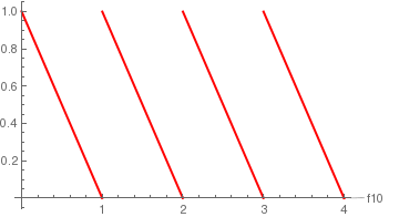
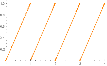
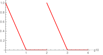
Example: Consider the function \( f(x) = 1-x \) on the interval [0,1]. To define its periodic extension, we use Mathematica command Mod:
f[t_]=1-t;
f10=periodicExtension[f,1,0];
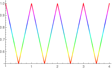
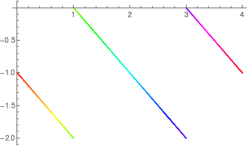
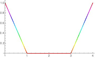
Plot[f10,{t,0,4}, PlotStyle -> {Thick, Red}, PlotLabels ->"Expressions"] f1 = periodicExtension[f,1];
Plot[f1,{t,0,4}, PlotStyle -> Thick, ColorFunction -> Function[{x,y}, Hue[y]]]
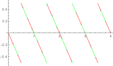
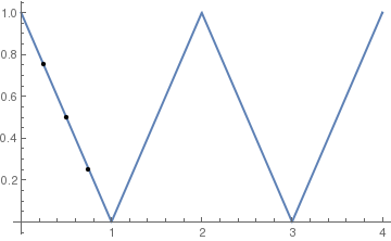
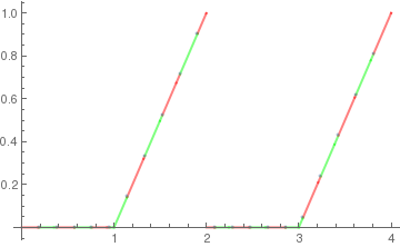
f12 = periodicExtension[f,1, 1/2];
Plot[f12,{t,0,4}, PlotStyle -> Directive[Opacity[0.5], Thick], Mesh ->20, MeshFunctions -> {#1 &}, MeshShading -> {Red, Green}]
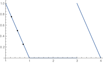
f1m1 = periodicExtension[f,1, -1];
Plot[f1m1,{t,0,4}, PlotStyle ->Orange, Mesh -> All]
f21 = periodicExtension[f,2,1];
Plot[f21,{t,0,4}, PlotStyle->Thick, ColorFunction -> Function[{x,y}, Hue[x]], ColorFunctionScaling->True]
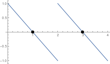
f20 = periodicExtension[f,2,0];
Plot[f20,{t,0,4}, PlotStyle->Thick, Epilog -> {PointSize[0.03], Point[{1,0}], Point[{3,0}]}]
f2m1 = periodicExtension[f,2,-1];
Plot[f2m1,{t,0,4}, PlotStyle -> Thick, Mesh ->{Range[0,1,1/4]}, MeshStyle ->PointSize[Medium]]
 |
 |
 |
 |
 |
 |
 |
To plot half-wave rectifiers, we need to define another piecewise continuous function
Plot[g10,{t,0,4}, PlotStyle -> {Thick, Red}, PlotLabels ->"Expressions"]
Plot[g4,{t,0,4}, PlotStyle -> Thick, ColorFunction -> Function[{x,y}, Hue[y]]]
g2m2 = periodicExtension[g,2, -2];
Plot[g2m2, {t,0,4}, PlotStyle -> Directive[Opacity[0.5], Thick], Mesh ->20, MeshFunctions -> {#1 &}, MeshShading -> {Red, Green}]
g30 = periodicExtension[g,3,0];
Plot[g30 ,{t,0,4}, PlotStyle -> Thick, Mesh ->{Range[0,1,1/4]}, MeshStyle ->PointSize[Medium]]
 |
 |
 |
 |
In each example below we start with a function defined on an interval, plotted in blue; then we present the periodic extension of this function, plotted in other color; then we present the Fourier expansion of this function, which is a Fourier periodic extension of the given function. The last figure in each example shows in one plot the Fourier expansion and the approximation with the partial sum with 20 terms of the corresponding Fourier series.
Example: Consider the following functions:
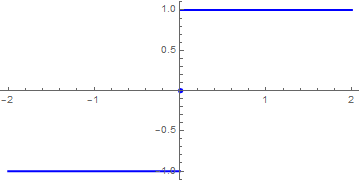
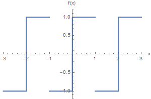
- \( f_1 (x) = \mbox{sign}(x)\,: \, (-1,1] \mapsto \, \mathbb{R}) \)
- \( f_2 (x) = x^2 \,: \, (1,4] \mapsto \, \mathbb{R} \)
We plot its periodic extension:
fbas[x_] := x^2 /; 1 <= x < 4
f[x_] := fbas[Mod[x, 3, 1]]
SetOptions[Plot, ImageSize -> 300];
Plot[f[x], {x, -3, 7}, PlotRange -> {-1.2, 16.2}, AxesLabel -> {"x", "f(x)"}, PlotStyle -> Thickness[0.01]]Function f2(x) is defined on the interval of length 3, so ℓ = 1.5. On symmetrical interval \( (-1.5,1.5) \) the given function can be written as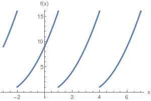 \[ f_2 (x) = \begin{cases} (x+3)^2 , & \ \mbox{for } -1.5 < x < 1 , \\ x^2 , & \ \mbox{for } 1 < x < 1.5 . \end{cases} \]To find its Fourier coefficients, we calculate the following integrals.a0 = 2*Integrate[(x + 3)^2, {x, -3/2, 1/2}]/3 + 2*Integrate[x^2, {x, 1, 3/2}]/3335/36an = Simplify[ 2*Integrate[(x + 3)^2 * Cos[2*n*Pi*x/3], {x, -3/2, 1/2}]/3 + 2*Integrate[x^2 *Cos[n*Pi*x*2/3], {x, 1, 3/2}]/3](1/(4 n^3 \[Pi]^3))(42 n \[Pi] Cos[(n \[Pi])/3] - 12 n \[Pi] Cos[(2 n \[Pi])/3] - 18 Sin[(n \[Pi])/3] + 49 n^2 \[Pi]^2 Sin[(n \[Pi])/3] + 18 Sin[(2 n \[Pi])/3] - 4 n^2 \[Pi]^2 Sin[(2 n \[Pi])/3] - 36 Sin[n \[Pi]] + 18 n^2 \[Pi]^2 Sin[n \[Pi]])bn = Simplify[ 2*Integrate[(x + 3)^2 * Sin[2*n*Pi*x/3], {x, -3/2, 1/2}]/3 + 2*Integrate[x^2 *Sin[n*Pi*x*2/3], {x, 1, 3/2}]/3](1/(4 n^3 \[Pi]^3))((18 - 49 n^2 \[Pi]^2) Cos[(n \[Pi])/3] + 2 ((-9 + 2 n^2 \[Pi]^2) Cos[(2 n \[Pi])/3] + 3 n \[Pi] (7 Sin[(n \[Pi])/3] - 2 Sin[(2 n \[Pi])/3] + 6 Sin[n \[Pi]])))Therefore, the required Fourier series for the function f2(x) becomes\[ f_2 (x) = \frac{335}{72} + \frac{1}{4 \pi^3} \sum_{n\ge 1} \frac{1}{n^3} \left\{ 42n\pi \,\cos \frac{n\pi}{3} -12n\pi \,\cos \frac{2n\pi}{3} + \left( 49 n^2 \pi^2 -18 \right) \sin \frac{n\pi}{3} + \left( 18 - 4n^2 \pi^2 \right) \sin \frac{2n\pi}{3} \right\} \cos \frac{2n\pi x}{3} + \frac{1}{4 \pi^3} \sum_{n\ge 1} \frac{1}{n^3} \left\{ \left( 18 -49 n^2 \pi^2 \right) \cos \frac{n\pi}{3} + 2 \left( 2n^2 \pi^2 -9 \right) \cos \frac{2n\pi}{3} + 42 n\pi\,\sin \frac{n\pi}{3} - 4\,\sin \frac{2n\pi}{3} \right\} \sin \frac{2n\pi x}{3} . \]Now we build its Fourier approximationfourier[m_] = a0/2 + Sum[an*Cos[2*n*Pi*x/3] + bn*Sin[2*n*Pi*x/3] , {n, 1, m}];and plot the corresponding sums with N = 10 and 20 terms:
ff10[x_] = 335/72 + Sum[an*Cos[2*n*Pi*x/3] + bn*Sin[2*n*Pi*x/3], {n, 1, 10}];
ff20[x_] = 335/72 + Sum[an*Cos[2*n*Pi*x/3] + bn*Sin[2*n*Pi*x/3], {n, 1, 20}];Plot[{ff10[x], ff20[x]}, {x, -2, 5}, PlotStyle -> {{Thick, Blue}, {Thick, Orange}}]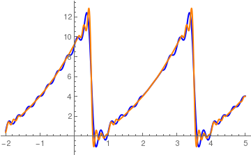
- \( \displaystyle f_3 (x) = \begin{cases} x , & \ \mbox{for } 0 < x < 2 , \\ 1, & \ \mbox{when } -2 < x < 0 .
\end{cases} \) This function maps the finite interval (-2,2) into \( \mathbb{R} . \)
We calculate the corresponding Fourier coefficients using Mathematica:
a0 = Integrate[1, {x, -2, 0}]/2 + Integrate[x, {x, 0, 2}]/22an = Simplify[ Integrate[Cos[n*Pi*x/2], {x, -2, 0}]/2 + Integrate[x *Cos[n*Pi*x/2], {x, 0, 2}]/2](-2 + 2 Cos[n \[Pi]] + 3 n \[Pi] Sin[n \[Pi]])/(n^2 \[Pi]^2)bn = Simplify[ Integrate[Sin[n*Pi*x/2], {x, -2, 0}]/2 + Integrate[x *Sin[n*Pi*x/2], {x, 0, 2}]/2]-((n \[Pi] + n \[Pi] Cos[n \[Pi]] - 2 Sin[n \[Pi]])/(n^2 \[Pi]^2))Therefore, the Fourier series becomes\[ f_3 (x) = 1 - \frac{4}{\pi^2} \sum_{k\ge 0} \frac{1}{(2k+1)^2} \,\cos \frac{(2k+1) \pi x}{2} - \frac{1}{\pi} \sum_{k\ge 1} \frac{1}{k}\,\sin (k\pi x) . \]Finally we build partial Fourier sums with 10 and 50 termsff10[x_] = 1 + 4/Pi^2 * Sum[1/(2*k+1)^2 * Cos[(2*k+1)*Pi*x/2], {k,0,10}] - Sum[1/k*Sin[k*Pi*x], {k,1,10}]/Pi; ff50[x_] = 1 + 4/Pi^2 * Sum[1/(2*k+1)^2 * Cos[(2*k+1)*Pi*x/2], {k,0,50}] - Sum[1/k*Sin[k*Pi*x], {k,1,50}]/Pi;and plot these approximationsPlot[{ff10[x], ff50[x]}, {x, -2, 5}, PlotStyle -> {{Thick, Blue}, {Thick, Orange}}]Since f3(0) = ½, we get a curious sum: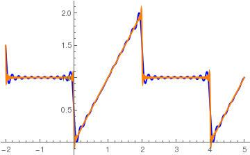 \[ \sum_{k\ge 0} \frac{1}{(2k+1)^2} = \frac{\pi^2}{8} \approx 1.2337. \]Mathematica also knows this sum:Sum[1/(2*k + 1)^2, {k, 0, Infinity}]\[Pi]^2/8
 - \( f_4 (x) = 1-|x|\,: \, (-2,2] \mapsto \, \mathbb{R} . \)
We first the corresponding Fourier coefficients
a0 = Integrate[(1-Abs[x]), {x, -2, 2}]/20an = Simplify[ Integrate[(1-Abs[x])*Cos[n*Pi*x/2], {x, -2, 2}]/2](4 - 4 Cos[n \[Pi]] - 2 n \[Pi] Sin[n \[Pi]])/(n^2 \[Pi]^2)bn = Simplify[ Integrate[(1-Abs[x])*Sin[n*Pi*x/2], {x, -2, 2}]/2]0Therefore, the given function f4 has the following Fourier cosine series\[ f_4 (x) = \frac{8}{\pi^2} \sum_{k\ge 0} \frac{1}{(2k+1)^2} \,\cos \frac{(2k+1) \pi x}{2} . \]Using Mathematica, we construct partial Fourier cosine sums and the periodic extension of the given function.ff10[x_] = 8/Pi^2 * Sum[1/(2*k+1)^2 * Cos[(2*k+1)*Pi*x/2], {k,0,10}];
ff50[x_] = 8/Pi^2 * Sum[1/(2*k+1)^2 * Cos[(2*k+1)*Pi*x/2], {k,0,50}];
per[x_] = Which[-2Plot[{ff10[x], per[x]}, {x, -2, 5}, PlotStyle -> {{Thick, Blue}, {Thick, Orange}}]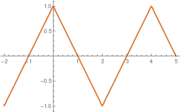
- \( f_5 (x) = \lfloor x \rfloor \,: \, (-2,2] \mapsto \, \mathbb{R} , \) where ⌊x⌋ is the floor function of x. Using its Fourier coefficients
■a0 = Integrate[Floor[x], {x, -2, 2}]/2-1an = Simplify[ Integrate[Floor[x]*Cos[n*Pi*x/2], {x, -2, 2}]/2]-(Sin[n \[Pi]]/(n \[Pi]))bn = Simplify[ Integrate[Floor[x]*Sin[n*Pi*x/2], {x, -2, 2}]/2](4 (2 + 3 Cos[(n \[Pi])/2]) Sin[(n \[Pi])/4]^2)/(n \[Pi])Hence, we get its Fourier series\[ f_5 (x) = - \frac{1}{2} + \frac{4}{\pi} \sum_{n\ge 1} \frac{1}{n} \left[ 2 + 3\,\cos \frac{n\pi}{2} \right] \sin^2 \frac{n\pi}{4} \,\sin \frac{n\pi x}{2} . \]Since the given function is a piecewise step functions, its Fourier series converges slowly showing Gibbs phenomenon at points of discontinuity (integer values).ff10[x_] = -1/2 +4/Pi * Sum[1/n * (2 + 3*Cos[n*Pi/2])*(Sin[n*Pi/4])^2 * Sin[n*Pi*x/2], {n,1,10}];Then we plot the approximation with N = 10 (blue) and 50 (orange) terms along with the given function (in black)):
ff50[x_] = -1/2 +4/Pi * Sum[1/n * (2 + 3*Cos[n*Pi/2])*(Sin[n*Pi/4])^2 * Sin[n*Pi*x/2], {n,1,50}];
per[x_] = Which[-2< x < 2,Floor[x], 2 < x < 6,Floor[x-4]]Plot[{ff10[x], ff50[x], per[x]}, {x, -2, 5}, PlotStyle -> {{Thick, Blue}, {Thick, Orange}, {Thick, Black}}]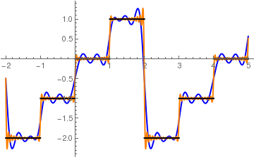
We describe periodic extension and its Fourier approximation in the following example.
Example: Consider the piecewise continuous function, defined on the interval \( [-2,2] . \)
\[ \left\{ \begin{array}{ll} 1 , & \ x<0 \\ x^2 , & \ x>0 \end{array} \right. \qquad\mbox{on the interval } (-2,2). \]To find its Fourier series, we calculate the corresponding Fourier coefficients:Clear[x,n,ak1,ak2,ak,bk1,bk2,bk,Sn]
ak1 = Integrate[1/2*Cos[n*Pi*x/2], {x,-2,0}];
ak2 = Integrate[1/2*x^2 * Cos[n*Pi*x/2], {x,0,2}];
bk1 = Integrate[1/2*Sin[n*Pi*x/2], {x,-2,0}];
bk2 = Integrate[1/2*x^2 * Sin[n*Pi*x/2], {x,0,2}];
ak = FullSimplify[ak1+ak2, Element[n, Integers]]
bk = FullSimplify[bk1+bk2, Element[n, Integers]]
a0 = FullSimplify[1/2* Integrate[1, {x,-2,0}] + 1/2 * Integrate[x^2 , {x,0,2}]]Out[6]= (8 (-1 + (-1)^n) - (1 + 3 (-1)^n) n^2 \[Pi]^2)/(n^3 \[Pi]^3)Now we define its periodic expansion. This could be achieved in many ways, and we give some approaches to find a periodic expansion.
Out[7]= (8 (-1)^n)/(n^2 \[Pi]^2)
Out[8]= 7/3f[x_] := Which[x > 2, f[x - 2*2], x < -2, f[x + 2*2], -2 < x < 0, 1 + x - x, 0 < x < 2, x^2]
Plot[f[x], {x, -5, 5}, PlotStyle -> {Thick, Black}]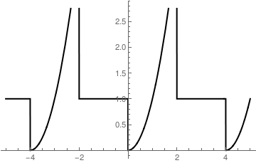
Other options to define periodic function:
f[x_] = Piecewise[{{1, x < 0}, {x^2, x > 0}}]Out[11]= \[ \left\{ \begin{array}{ll} 1 & \ x<0 \\ x^2 & \ x>0 \\ 0 & \ \mbox{True} \end{array} \right. \]
We define a subroutine that provide periodic extension of a function:
myperiodic[func_, {val_Symbol, min_?NumberQ, max_?NumberQ}] := func /. (val :> Mod[val - min, max - min] + min)Then we plot it:Plot[myperiodic[f[x], {x, -2, 2}] // Evaluate , {x, -5, 5}, PlotStyle -> {Thick, Black}]We demonstrate other options to determine a periodic extension on our old piecewise continuous function.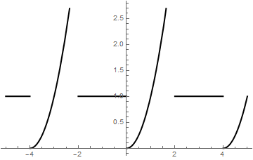 Clear[f];
f[x_] = Piecewise[{{1, x < 0}, {x^2, x > 0}}]
f[t_ /; t >= 2] := f[t - 4]; f[t_ /; t < -2] := f[t + 4]; Plot[f[t], {t, -10, 10}] , PlotStyle -> {Thick}]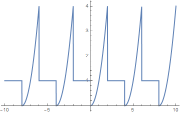 f[x_] = Piecewise[{{1, x < 0}, {x^2, x > 0}}]
g[x_] = f@Mod[x, 4 , -2] (* somehow slow *)
Plot[{f[t], g[t]}, {t, -6, 6}, PlotStyle -> Thick]A periodic extension can be defined for arbitrary period as the following example shows.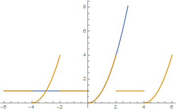 T = 2.5
g[x_ /;0<= x <= T] := x^2 +1;
f[x_] := g[Mod[x, T]]
Plot[f[t], {t, -6, 6}, PlotRange -> {{-5,5}, {-0.1, 8}}, PlotStyle -> Thick]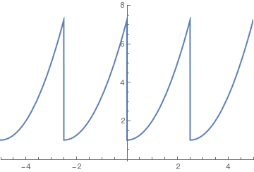
Example: Consider the following function that we met previously
\[ f(x) = \left\{ \begin{array}{ll} \cos x, & \ \mbox{within interval $[-\pi /2 , \pi /2 ]$}, \\ 0 , & \ \mbox{outside the interval within } [-\pi , \pi ]. \end{array} \right. \]We can also define the periodic expansion of any function using Mod command. If we need to define a function with period \( 2*\pi , \) we type:
periodicExtension[func_] := func[Abs[Mod[t, 2*Pi, -1*Pi]]]
per = periodicExtension[f]Out[2] = { Cos[Abs[Mod[t,2*Pi , -Pi]]] -Pi/2 < Abs[Mod[t, 2*Pi , -Pi]] < Pi/2
0 TruePlot[per, {t, -10, 10}, PlotStyle -> Thick]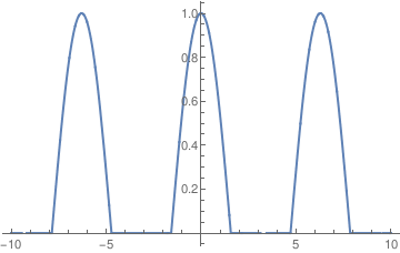 FourierTrigSeries[f[t], t, 5]Out[6] = 1/\[Pi] + Cos[t]/2 + (2 Cos[2 t])/(3 \[Pi]) - (2 Cos[4 t])/(15 \[Pi])Plot[%, {t, -3*Pi, 3*Pi}, PlotStyle -> Thick, AspectRatio -> 1/5]
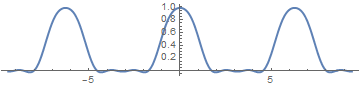
- Gregory A. Kriegsmann, A mathematical theory of full-wave rectification, IMA Journal of Applied Mathematics, Volume 36, Issue 1, 1 January 1986, Pages 29--41, https://doi.org/10.1093/imamat/36.1.29
- C. Marouchos ; M.K. Darwish ; M. El-Habrouk, New mathematical model for analysing three-phase controlled rectifier using switching functions, IET Power Electronics, Volume: 3, Issue: 1, January 2010, 95--110. doi: 10.1049/iet-pel.2008.0328
- Le Hong Lan and Nguyen Thi Hien, Mathematical model written by the canonical system for some electric rectifier circuits using semiconductor diodes, article
- Branco Curgus, Fourier periodic extensions of piecewise continuous functions, http://faculty.wwu.edu/curgus/Courses/Math_pages/Math_430/Fourier_periodic_extension.html
- Mohammed A. Abbas, Falah H.Hanoon, and Lafy F.Al-Badry, Possibility designing half-wave and full-wave molecular rectifiers by using single benzene molecule, Physics Letters A, Volume 382, Issue 8, 27 February 2018, Pages 608--612. https://doi.org/10.1016/j.physleta.2017.12.017
Return to Mathematica page
Return to the main page (APMA0340)
Return to the Part 1 Matrix Algebra
Return to the Part 2 Linear Systems of Ordinary Differential Equations
Return to the Part 3 Non-linear Systems of Ordinary Differential Equations
Return to the Part 4 Numerical Methods
Return to the Part 5 Fourier Series
Return to the Part 6 Partial Differential Equations
Return to the Part 7 Special Functions - \( f_5 (x) = \lfloor x \rfloor \,: \, (-2,2] \mapsto \, \mathbb{R} , \) where ⌊x⌋ is the floor function of x. Using its Fourier coefficients
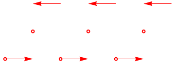
b = Graphics[{Blue, Thick, Circle[{0, 0}, 0.02]}, AspectRatio -> 1]
Show[a, b]
b = Graphics[{Red, Arrowheads[0.05], Arrow[{{1, 1}, {0, 1}}]}]
c = Graphics[{Red, Thick, Circle[{0, 0}, 0.05]}, AspectRatio -> 1/2]
b2 = Graphics[{Red, Arrowheads[0.05], Arrow[{{3, 1}, {2, 1}}]}]
a1 = Graphics[{Red, Arrowheads[0.05], Arrow[{{1, -1}, {2, -1}}]}]
c2 = Graphics[{Red, Thick, Circle[{2, 0}, 0.05]}, AspectRatio -> 1/2]
a3 = Graphics[{Red, Arrowheads[0.05], Arrow[{{3, -1}, {4, -1}}]}]
ac = Graphics[{Red, Thick, Circle[{-1, -1}, 0.05]}, AspectRatio -> 1/2]
ac1 = Graphics[{Red, Thick, Circle[{1, -1}, 0.05]}, AspectRatio -> 1/2]
ac3 = Graphics[{Red, Thick, Circle[{3, -1}, 0.05]}, AspectRatio -> 1/2]
c4 = Graphics[{Red, Thick, Circle[{4, 0}, 0.05]}, AspectRatio -> 1/2]
b4 = Graphics[{Red, Arrowheads[0.05], Arrow[{{5, 1}, {4, 1}}]}]
Show[a, b, c, c2, b2, a1, a3, ac, ac1, ac3, c4, b4]
 |
 |
fbas[x_] := 1 /; 0 <= x < L
L = 1;
f[x_] := fbas[Mod[x, 2*L, -L]]
SetOptions[Plot, ImageSize -> 300];
Plot[f[x], {x, -3*L, 3*L}, PlotRange -> {-1.2, 1.2}, AxesLabel -> {"x", "f(x)"}, PlotStyle -> Thickness[0.008]]
(1) adds L to x,
(2) calculates the remainder on dividing (1) by 2*L,
(3) subtracts L from (2). This has the effect of shifting the original x by ±2L until it falls into the range [-L,L). This modified x is then used as the argument of the original function f[x].
We plot the periodically extended function over three periods -- that is over [-3L, 3L].
Strictly speaking the vertical lines shown on the graph at the discontinuity are not part of the graph. In some ways they make it easier to visualize the discontinuous function, but on those days when we are feeling fussy, we can exclude those segments. This is done by an Option for plot called Exclusions. The plot without the vertical lines is constructed below. The argument of the Option Exclusions is a list of points to be excluded.
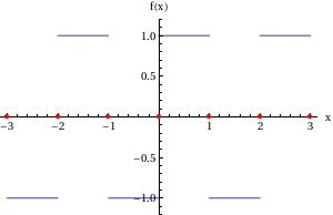
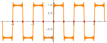
A=Plot[f, {x, -5, 5}, PlotStyle -> {Thick, Orange}, AspectRatio -> 2/5]
cm1 = Graphics[{Red, Thick, Disk[{-1, 0}, 0.07]}, AspectRatio -> 1/4]
Show[A, c4, c3, c2, c1, c0, cm1, cm2, cm3, cm4]