Preface
A nonholonomic system is a system whose state depends on the path taken in order to achieve it. Such a system is described by a set of parameters subject to differential constraints, such that when the system evolves along a path in its parameter space (the parameters varying continuously in values) but finally returns to the original set of parameter values at the start of the path, the system itself may not have returned to its original state.
Return to computing page for the first course APMA0330
Return to computing page for the second course APMA0340
Return to Mathematica tutorial for the first course APMA0330
Return to Mathematica tutorial for the second course APMA0340
Return to the main page for the first course APMA0330
Return to the main page for the second course APMA0340
Introduction to Linear Algebra with Mathematica
Glossary
Lagrange multipliers for n-dimensional case
Thus, we solve the equation \( \nabla f = 0 , \) which is equivalent to the system of algebraic equations
Lagrange Multipliers
For nonholonomic systems, the generalized coordinates qi are not independent of each other and it is impossible to reduce them by means of constraint equations. However, if there are k constraints of the form \( \sum_{k=1}^{3n} A_{jk} \,\delta q_k =0 , \) where \( j =1,2,\ldots , k ; \) then Lagrange multipliers can be used to describe the constraints. The equations of motion that follow from these constraints are
The Lagrange multiplier by itself has no physical meaning: it can be transformed into a new function of time just by rewriting the constraint equation into something physically equivalent.
Let us consider the general problem of finding the extremum of a functional
Example: Let us consider the case of a block sliding down a fixed frictionless incline of angle θ. Obviously, the easiest approaches to this would be to either just write down Newton's 2nd law in a convenient coordinate system or to use the generalized coordinate q representing the distance traveled along the incline by the block and just writing down Lagrange's equations. For the second method, the choice of generalized coordinate q will implicitly take into account the constraint which is that the block must stay on the incline during the trajectory before reaching the ground. However, let's do this using the method of Lagrange multipliers.
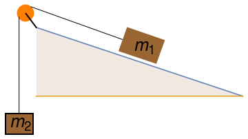
Using x for the horizontal coordinate and y for the vertical coordinate, we can write out Lagrangian as \( L = \frac{1}{2}\, m\,\dot{x}^2 + \frac{1}{2}\, m\,\dot{y}^2 + mgy . \) However, the rectangular coordinates are not independent: they are related by the holonomic constraint \( g(x,y) = y - x\,\tan \theta . \) Setting \( L' = L- \lambda\,g , \) we apply Lagrange's second equation
Now assume that there is a friction acting on mass m1, which we model as
- J. R. Gaskill Jr. and M. Arenstein, Geometrical View of Lagrange Multipliers in Mechanics, Journal of Mathematical Physics, 8, Issue 9, 1912 (1967); https://doi.org/10.1063/1.1705436
- Volkov, A. and Zubelevich, O., Lagrangian systems with non-smooth constraints, Glasgow Mathematical Journal, 2016, Vol. 59, No. 2, pp. 289--298; doi: 10.1017/S0017089516000173
Return to Mathematica page
Return to the main page (APMA0340)
Return to the Part 1 Matrix Algebra
Return to the Part 2 Linear Systems of Ordinary Differential Equations
Return to the Part 3 Non-linear Systems of Ordinary Differential Equations
Return to the Part 4 Numerical Methods
Return to the Part 5 Fourier Series
Return to the Part 6 Partial Differential Equations
Return to the Part 7 Special Functions