The gamma function Γ(x) is the natural extension of the factorial function \( n! = \prod_{k=1}^n k = 1 \cdot 2 \cdot 3 \cdots n \) from integer n to real or complex x.
It was first defined and studied by L. Euler in 18th century, who used the notation Γ(z), the capital letter gamma from the Greek alphabet. It is commonly used in many mathematical problems, including differential equations, but it appears occasionally in physical problems such as the normalization
of Coulomb wave functions and the computation of probabilities in statistical mechanics.
In general, however, it has less direct physical application and interpretation than, say, the
Chebyshev and Bessel functions. Rather, its importance stems from its
usefulness in developing other functions that have direct physical application.
The first definition, given by Leonhard Euler is
\[
\Gamma (z) = \lim_{n\to \infty} \,\frac{n!}{z\left( z+1 \right) \left( z+2 \right) \cdots \left( z+n \right)} , \qquad z\ne 0, -1, -2, \ldots .
\]
This definition is not very useful in differential equations. The more common way to define the gamma function is through the following integral:
\begin{equation} \label{EqGamma.1}
\Gamma (\nu ) = \int_0^{\infty} t^{\nu -1} e^{-t} {\text d} t , \qquad \Re (\nu ) > 0.
\label{EqGamma.1}
\end{equation}
The restriction on ν is necessary to avoid divergence of the integral.
Mathematica uses the conventional notation:
Gamma[ν].
There are known several equivalent definitions of the gamma function:
\begin{equation}
\Gamma (\nu ) = 2 \int_0^{\infty} t^{2\nu -1} e^{-t^2} {\text d} t = \int_0^1 \left[ \ln \left( \frac{1}{t} \right) \right]^{\nu -1} {\text d} t .
\label{EqGamma.2}
\end{equation}
Mathematica uses the conventional notation:
Gamma[ν, x].
|
|
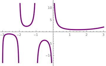
Mathematica has a dedicated command for the gamma function -- Gamma[ z ].
You can make a fancy plotof this function:
Plot[Gamma[x], {x, -3, 3}, PlotStyle -> {Purple, Thickness[0.01]}]
The gamma function has a local minimum at +1.46163214496836234126.
|
|
The Gamma function.
|
|
Mathematica code
|
When ν = ½, Eq.\eqref{EqGamma.1} is just the Gauss erroe integral
\( \Gamma (1/2) = \sqrt{\pi} . \) In general, we have
\begin{equation}
\Gamma \left( \frac{1}{2} + n \right) = \frac{(2n)!}{4^n n!}\,\sqrt{\pi} = \frac{(2n-1)!!}{2^n} \,\sqrt{\pi} \qquad\mbox{and} \qquad \Gamma \left( \frac{1}{2} - n \right) = \frac{(-4)^n n!}{(2n)!}\,\sqrt{\pi} = \frac{(-2)^n}{(2n-1)!!} \,\sqrt{\pi} .
\label{EqGamma.3}
\end{equation}
One of the most important properties of the gamma function is its recurrence relation (difference equation of the first order)
\begin{equation}
\Gamma (\nu +1) = \nu\,\Gamma (\nu ) , \qquad \Gamma (1) = \Gamma (2) = 1.
\label{EqGamma.4}
\end{equation}
This leads to the remarkable formula that generalizes the factorial:
\begin{equation}
\Gamma (n +1) = 1 \cdot 2 \cdot 2 \cdots n = n! \qquad\mbox{for integer} \quad n \ge 0.
\label{EqGamma.5}
\end{equation}
Other important functional equations for the gamma function are Euler's reflection formula
\begin{equation}
\Gamma \left( 1-z \right) \Gamma (z) = \frac{\pi}{\sin (\pi z)} , \qquad z \notin \mathbb{Z} .
\label{EqGamma.6}
\end{equation}
|
|
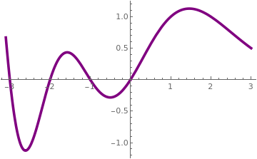
With Mathematica, one can plot the reciprocal of the gamma functions:
Plot[1/Gamma[x], {x, -3.1, 3}, PlotStyle -> {Purple, Thickness[0.01]}]
|
|
The reciprocal of the Gamma function.
|
|
Mathematica code
|
Incomplete gamma function
The upper incomplete gamma function is defined as:
\[
\Gamma (\nu , x) = \int_x^{\infty} t^{\nu -1} e^{-t} {\text d} t ,
\]
whereas the lower incomplete gamma function is defined as:
\[
\gamma (\nu , x) = \int_0^x t^{\nu -1} e^{-t} {\text d} t .
\]
Clearly, the two functions are related, for
\[
\gamma (\nu , x) + \Gamma (\nu , x) = \Gamma (\nu ) .
\]
Mathematica uses the notation:
Gamma[ν, 0, x] for the lower incomplete gamma function.
The gamma function is related to the beta function by the formula
\[
B(x,y) = \int_0^1 t^{x-1} \left( 1- t \right)^{y-1} {\text d} t = \frac{\Gamma (x)\,\Gamma (y)}{\Gamma (x+y)} .
\]
the
digamma function is defined as the logarithmic derivative of the gamma function
\[
\psi (x) = \frac{\text d}{{\text d}x} \, \ln \left( \Gamma (x) \right) = \frac{\Gamma' (x)}{\Gamma (x)} .
\]
Then the derivatives of the gamma function are described in terms of the polygamma function
\[
\Gamma' (z) = \Gamma (z)\,\psi_0 (z)
\]
The recurrence relation for the digamma function is
\[
\psi (z+1) = \psi (x) + \frac{1}{z} .
\]
This allows to relate the digamma function for integers and the the
harmonic numbers:
\[
H_n = 1 + \frac{1}{2} + \cdots + \frac{1}{n} = \sum_{k=1}^n \frac{1}{k} = \psi (n+1) + \gamma ,
\]
where γ = 0.57721566490153286060651209008240243104215933593992... is the
Euler constant (also known as Euler–Mascheroni constant).
the
exponential integral Ei is a special function on the complex plane ℂ:
\[
\mbox{Ei}(z) = - \int_{-x}^{\infty} \frac{e^{-t}}{t}\,{\text d} t = \int_{-\infty}^x \frac{e^{t}}{t}\,{\text d} t
\]
Return to Mathematica page
Return to the main page (APMA0340)
Return to the Part 1 Matrix Algebra
Return to the Part 2 Linear Systems of Ordinary Differential Equations
Return to the Part 3 Non-linear Systems of Ordinary Differential Equations
Return to the Part 4 Numerical Methods
Return to the Part 5 Fourier Series
Return to the Part 6 Partial Differential Equations
Return to the Part 7 Special Functions