Return to computing page for the first course APMA0330
Return to computing page for the second course APMA0340
Return to computing page for the fourth course APMA0360
Return to Mathematica tutorial for the first course APMA0330
Return to Mathematica tutorial for the second course APMA0340
Return to Mathematica tutorial for the fourth course APMA0360
Return to the main page for the first course APMA0330
Return to the main page for the second course APMA0340
Return to the main page for the fourth course APMA0360
Return to Part V of the course APMA0340
Introduction to Linear Algebra with Mathematica

Preface


Our presentation of Fourier series in this section is not done in great depth or generality to meet the pure mathematician's criteria for accuracy. For example, we utilize Riemann integration in the majority of proofs rather than Lebesgue's one in order to make all concepts friendly accessible. Also, maximum is used for definition of uniform norm instead of "supremum" because it is sufficient in most applications. Our exposition is intended as a shop window for basic ideas, techniques, and elegant results of Fourier analysis, with suggested references for further study.

Although there are many methods for signal representations, Fourier analysis involving the resolution of signals into sinusoidal components dominates. Periodic signals occur in a wide range of physical phenomena, a few examples of which are acoustic and electromagnetic waves, periodic vibrations of musical instruments, vertical displacement of a mechanical pendulum, and periodic signals in electrical engineering. From theoretical or mathematical point of view, a Fourier series of a function is its spectral decomposition with respect to orthogonal basis formed by eigenfunctions corresponding to a Sturm--Liouville problem.

This section presents a particular application of eigenfunction expansion corresponding to the regular Sturm--Liouville problem with periodic condition,

\[ \hat{p}\,u = %L_1 \left[ \texttt{D} \right] u = \mu\, u(x) \qquad \Longleftrightarrow \qquad {\bf j}\,u' + \mu\, u(x) =0, \qquad u(-\ell ) = u(\ell ) , \]
where the momentum operator \( \hat{p} = -{\bf j}\,\texttt{D} = -{\bf j}\,{\text d}/{\text d}x \) is the first order self-adjoint differential operator with j being the unit vector along the positive vertical direction on the complex plane ℂ, so j² = −1. As usual, we use Lagrange's notation for the derivative: \( \quad y' = {\text d}y/{\text d}x . \) The formulated problem contains a parameter μ, and it asks to determine the values of the parameter for which the problem has nontrivial (not identically zero) solutions. Such values of parameter μ are referred to as eigenvalues, and corresponding solutions are called eigenfunctions.

The general solution of the differential equation \( \quad {\bf j}\,u'(x) + \mu\, u(x) =0 \) is \( u(x) = C\,e^{{\bf j}\mu x} , \) for some constant C. To satisfy the periodic boundary condition, we have to set μ = nπ/ℓ for some integer n ∈ ℤ = { 0, ±1, ±2, …}. So the eigevalues for this first order differential equation are \( \mu_n = \frac{n\pi}{\ell} , \quad n = 0, \pm 1, \pm 2, \ldots , \) to which correspond eigenfunctions \( u_n (x) = e^{{\bf j}\pi n x/\ell} , \) up to some nonzero constant multiple.

Instead of the first order differential operator \( \hat{p} = -{\bf j}\,\texttt{D} = -{\bf j}\,{\text d}/{\text d}x \) with complex coefficient j, it is convenient to square it in order to get rid of the coefficient. Therefore, the corresponding Sturm--Liouville problem with a parameter λ can be written in the form:

\[ L_2 \left[ \texttt{D} \right] y = \lambda\,y(x) \qquad \Longleftrightarrow \qquad y'' +\lambda\,y(x) = 0 , \qquad y(-\ell ) = y(\ell ) , \quad y'(-\ell ) = y'(\ell ) , \]
where λ is a nonnegative number and \( L_2 \left[ \texttt{D} \right] = - \texttt{D}^2 = \left( -{\bf j}\texttt{D} \right)^2 = \left( \hat{p} \right)^2 \) is the second order differential operator with \( \texttt{D} = {\text d}/{\text d}x . \) In physics, this operator is called Hamiltonian and it is denoted by Ĥ. The problem assumes that its solution y(x) is a real-valued function defined on a symmetric interval (chosen for simplicity, without any loss of generality) of length T = 2ℓ. Because of periodic boundary conditions, the function y(x) can be considered only on this finite interval, assuming that y(x + T) = y(x) for all x ∈ ℝ. As it was shown in the openning section, the self-adjoint operator \( L_2 \left[ \texttt{D} \right] = - \texttt{D}^2 \) has an infinite discrete set of nonnegative/positive eigenvalues \( \lambda_k = \left( \frac{k\pi}{\ell} \right)^2 , \quad k=0,\pm 1, \pm 2,\ldots ; \) therefore, L2 is called a nonnegative/positive operator.

Since the differential operator L2 is a square of of the first order momentum operator \( L_2 \left[ \texttt{D} \right] = \hat{p}^2 , \) its eigenvalues must be squares of the latter:

\[ \lambda_k = \left( \frac{k\pi}{\ell} \right)^2 = \mu_k^2 , \qquad k=0, \pm 1, \pm 2, \ldots . \]
Therefore, eigenvalues λk = λ−k collide for positive and negative indices. However, their eigenfunctions don't, and we have the sequence of real-valued eigenfunctions:
\[ \phi_k (x) = \cos \left( \frac{k\pi x}{\ell} \right) , \quad k=0,1,2,\ldots ; \qquad \phi_{-k} (x) = \sin \left( \frac{k\pi x}{\ell} \right) , \quad k=1,2,\ldots . \]

Often, eigenfunctions are organized in two-dimensional vector form:

\[ \left\{ \left[ \begin{array}{c} 1 \\ 0 \end{array} \right] , \ \left[ \begin{array}{c} \cos \frac{\pi x}{\ell} \\ \sin \frac{\pi x}{\ell} \end{array} \right] , \ \left[ \begin{array}{c} \cos \frac{2\pi x}{\ell} \\ \sin \frac{2\pi x}{\ell} \end{array} \right] , \ \left[ \begin{array}{c} \cos \frac{3\pi x}{\ell} \\ \sin \frac{3\pi x}{\ell} \end{array} \right] , \cdots \left[ \begin{array}{c} \cos \frac{n\pi x}{\ell} \\ \sin \frac{n\pi x}{\ell} \end{array} \right] , \cdots \right\} . \]
The Sturm--Liouville problems formulated above can be written in operator form
\[ L \left[ \texttt{D} \right] y = \lambda\,y , \qquad y(-\ell ) = y(\ell ) , \]
where L is one of the following differential operators:
\[ L_2 \left[ \texttt{D} \right] = - \texttt{D}^2 \qquad \mbox{or} \qquad \hat{p} = -{\bf j}\,\texttt{D} , \qquad\mbox{with} \quad \texttt{D} = {\text d}/{\text d}x . \]
Actually, these two differential operators are related:
\[ L_2 \left[ \texttt{D} \right] = \left( \hat{p} \right)^2 \qquad \mbox{or} \qquad - \texttt{D}^2 = \left( - {\bf j}\,\texttt{D} \right)^2 = {\bf j}^2 \texttt{D}^2 , \qquad {\bf j}^2 -1. \]
As it was shown in the previous section, the unbounded linear operator L2 with periodic condition is a non-negative operator, meaning that all its eigenvalues are not negative.

Any eigenvalue problem can be written in abstract way as \( L\, y = \lambda\,y , \) which is actually a spectral representation of the linear operator L. The idea of such representation is to reduce action of the operator L on a function to multiplication operation. In contrast to finite dimensional case (matrices), an unbounded operator has infinite many (maybe continuous) eigenvalues.

Assuming λ≥0, we solve the Sturm--Liouville problem for L2.

\[ y'' + \lambda\,y = 0, \qquad y(-\ell ) = y(\ell ) \quad y'(-\ell ) = y'(\ell ) . \]
The general solution of the differential equation depends on two arbitrary real constants c1 and c2:
\[ y(x) = c_1 \cos \left( \sqrt{\lambda}\,x \right) + c_2 \sin \left( \sqrt{\lambda}\,x \right) . \]
This function can be periodic with period T if and only if
\[ \sqrt{\lambda} = \frac{2\pi n}{T} \qquad \Longrightarrow \qquad \lambda_n = \left( \frac{2\pi n}{T} \right)^2 , \quad n=0,1,2,\ldots . \]
It is a custom to set the period to be an even number: T = 2ℓ. Then due to periodicity of the problem, it is also convenient to consider a symmetric interval [−ℓ, ℓ] because any interval of length T = 2ℓ can be used.

The first order differential operator \( \hat{p} \) acts on complex-valued functions (as well as on real-valued functions). The general solution of \( {\bf j}\,u' + \mu\, u = 0 \) depends on one arbitrary complex number A = 𝑎 + jb (where 𝑎 and b are real numbers):

\[ u(x) = A\, e^{{\bf j}\mu x} = \left( a + {\bf j}b \right) e^{{\bf j}\mu x} = \left( a + {\bf j}b \right) \left( \cos \mu x + {\bf j}\,\sin \mu x \right) . \]
The function u(x) is a periodic function (independently on A) when
\[ \mu = \mu_n = \frac{n2\pi}{T} , \qquad n= 0,\pm 1, \pm 2,\ldots . \]
Note that since \( L_2 \left[ \texttt{D} \right) = \left( -{\bf j}\,\texttt{D} \right)^2 , \) their eigenvalues are related
\[ \lambda_n = \mu_n^2 = \left( \frac{2\pi n}{T} \right)^2 , \quad n=0,\pm 1, \pm 2,\ldots . \]
Finally, we get a sequence of eigenfunctions corresponding to eigenvalues μn:
\[ u_n (x) = A_n e^{2{\bf j}n\pi x/T} , \qquad \mbox{where} \quad T = 2\ell . \]

﹡ ⁎ ✱ ✲ ✳ ✺ ✻ ✼ ✽ ❋

An essential part of the Sturm--Liouville theory includes function expansions with respect to the (infinite) system of eigenfunctions---a complete set for every self-adjoint differential operator of the second order. The majority of applications of the Sturm--Liouville theory utilizes expansions of a function f(x) that satisfies the homogeneous boundary conditions (in our case, they are periodic conditions)

\begin{equation} \label{EqFourier.0} f(x) = \sum_k c_k \phi_k (x) , \end{equation}
where ϕk(x) are eigenfunctions for either second order operator \( L_2 \left[ \texttt{D} \right] = - \texttt{D}^2 \) or momentum operator \( \hat{p} = - {\bf j} \texttt{D} . \) The coefficients ck = ck(f) of the expansion, \( f(x) = \sum_k c_k \phi_k (x) , \) for a function f(x) over the set of eigenfunctions {ϕk(x)} are called the Fourier coefficients. An ordered list of Fourier coefficients can be considered as a vector in infinite dimensional space spanned on eigenfunctions. We prefer to use Dirac's's notation for identification of this discrete list of Fourier coefficients:
\[ \vert\, f \,\rangle = \left[ \cdots , c_{-n} , \cdots , c_0 , c_1 , c_2 , \cdots , c_n , \cdots \right] . \]

Since every eigenfunction ϕk(x) in decomposition \eqref{EqFourier.0} satisfies the periodic condition, we expect that the function f(x) also matches this condition, so we require that f(−ℓ) = f(ℓ). Anyway, the Fourier expansion \eqref{EqFourier.0} assigns numerical values at endpoints for f(x). If the values of f(x) at the endpoints do not match, then this just means that there is a discontinuity at that point---don't worry, the Fourier series will correct you. Hence, the Fourier series dictates the determination of f at endpoints according to the average of its one sided limits:

\[ f(-\ell ) = f(\ell ) = \frac{1}{2} \left[ f(-\ell +0) + f(\ell -0) \right] = \lim_{\varepsilon \downarrow 0} \frac{1}{2} \left[ f(-\ell +\varepsilon ) + f(\ell -\varepsilon ) \right] . \]
In many applications, particular values of f(x) at endpoints do not matter because function f(x) is specified on an open interval (−ℓ, ℓ) rather than closed interval. Actually, the Fourier series assigns numerical values at every point of the closed interval [−ℓ, ℓ], including endpoints. Pointwise convergence of series \eqref{EqFourier.0} is discussed in convergence section and other issues of convergence in mean convergence section.

Definition of Fourier Series


Historically, Fourier series was a first example of expansions with respect to eigenfunctions corresponding to a Sturm--Liouville problem with periodic boundary conditions. Since a function to be decomposed into Fourier series should match thess boundary conditions, we assume that this function is a periodic function. In addition, we assume that all periodic functions have period T = 2ℓ, without any loss of generality. Therefore, it is sufficient to consider real-valued functions f : [−ℓ, ℓ] → ℝ with the values at endpoints \( f(-\ell ) = f(\ell ) = \frac{1}{2} \left[ f(-\ell + 0) + f(\ell -0) \right] \) to match the periodicity condition.

Every expansion can be written in the series form \eqref{EqFourier.0}. Therefore, it includes two mutually depending ingredients: Fourier coefficients {ck} and the set of eigenfunctions { ϕk }. Mathematicians proved (because Sturm and Liouville did not demonstrate existence of eigenvalues and eigenfunctions) that an unbounded self-adjoint differential operator of second order subject to some homogeneous boundary conditions possesses a discrete set of eigenvalues and corresponding eigenfunctions. Synthesizing function f(x) from its discrete list | f ⟩ of Fourier coefficients is referred to as the Fourier series for function f(x). In other words, the Fourier series of a function f(x) is its decomposition into periodic waves---one of the most useful concepts in physics, and features in many branches of engineering. Restoring the function from its Fourier coefficients is an ill-posed problem.

There are two equivalent forms of Fourier series based on two eigenfunction expansions corresponding to the first order operator \( \hat{p} = - {\bf j}\,\texttt{D} \) and the second order operator \( L_2 \left[ \texttt{D} \right] = - \texttt{D}^2 = \left( -{\bf j} \texttt{D} \right)^2 = \left( \hat{p} \right)^2 = \hat{H}(p) . \) The former one provides an eigenfunction expansion in a complex form (or exponential form)

\begin{equation} \label{EqFourier.1} f(x) \,\sim\, \mbox{P.V.}\sum_{n=-\infty}^{\infty} \hat{f}(n)\, e^{n{\bf j} \pi x/\ell} = \lim_{N\to \infty} \sum_{n=-N}^{N} \hat{f}(n)\, e^{n{\bf j} \pi x/\ell} = S[f](x) , \end{equation}
where T = 2ℓ is the period and x is a real variable. As usual, j is the unit (imaginary) vector on complex plane ℂ, so j² = −1. Here «P.V.» abbreviates the Cauchy principal value, which is a regularization of the infinite summation. Since this series may or may not converge, and if it converges, we don't know whether its sum is f(x), we cannot write \( f(x) \,=\, \sum_{n=-\infty}^{\infty} \hat{f}(n)\, e^{n{\bf j} \pi x/\ell} . \) Hence, we use a tilde (∼) instead of equal symbol (=) simply to denote the fact that the Fourier coefficients \( \hat{f}(n) \) are evaluated according to the Euler--Fourier formulas:
\begin{equation} \label{EqFourier.2} \hat{f}(n) = \frac{1}{2\ell} \int_{-\ell}^{\ell} f(x)\, e^{-n{\bf j} \pi x/\ell} \,{\text d} x = \frac{1}{T} \int_{0}^{T} f(x)\, e^{-2n{\bf j} \pi x/T} \,{\text d} x , \qquad n \in \mathbb{Z} = \left\{ 0, \pm 1, \pm 2, \ldots \right\} . \end{equation}
This means that the function f(x) is expanded into formal series \eqref{EqFourier.1} that is convenient to denote the latter by S[f]. Since a restoration of the function f(x) from its Fourier coefficients \eqref{EqFourier.2} is an ill-posed problem, a natural definition of two-sided infinite series (that you learnt in calculus)
\[ \sum_{n=-\infty}^{+\infty} \hat{f}(n)\, e^{n{\bf j} \pi x/\ell} = \lim_{N.M \to +\infty} \sum_{n=-M}^{N} \hat{f}(n)\, e^{n{\bf j} \pi x/\ell} \]
does not work in many cases.

Example 1: We expand the following complex-valued function into exponential Fourier series:

\[ \pi\, e^{{\bf j}\left( \pi -x \right) \alpha} \,\sim \mbox{P.V.\ \ } e^{{\bf j}\alpha\pi} 2\sum_{n=-\infty}^{\infty} \frac{\sin \left( n + \alpha \right) \pi}{n+\alpha}\, e^{{\bf j}nx} . \]
Indeed, its Fourier coefficients are
\[ \hat{f} (n) = \frac{1}{\pi} \int_{-\pi}^{\pi} \pi\, e^{{\bf j}\left( \pi -x \right) \alpha} \, e^{-{\bf j}nx} {\text d} x = \frac{2\,\sin \left( n+ \alpha \right) \pi}{\left( n + \alpha \right)}\, e^{{\bf j}\alpha\pi} . \]
Simplify[Integrate[Exp[-I*n*x + I*(Pi - x)*alpha], {x, -Pi, Pi}]] Pi/Sin[Pi*alpha]
-((I E^(-I n \[Pi]) (-1 + E^(2 I (alpha + n) \[Pi])))/(alpha + n)) alpha \[Pi]])/(alpha + n)
When α = ½, we have
\[ \pi\, e^{{\bf j}\left( \pi -x \right) /2} = 2\, e^{{\bf j}\pi /2} \sum_{n=-\infty}^{\infty} \frac{\sin \left( n + \frac{1}{2} \right) \pi}{n+\frac{1}{2}}\, e^{{\bf j}nx} . \]
Separation of real and imaginary parts yields
\begin{align*} \Re \pi\, e^{{\bf j}\left( \pi -x \right) /2} &= \pi \sin \left( \frac{x}{2} \right) = -8 \sum_{n\ge 1} \frac{n (-1)^n}{4 n^2 -1} \,\sin (nx) , \\ \Im \pi\, e^{{\bf j}\left( \pi -x \right) /2} &= \pi \cos \left( \frac{x}{2} \right) = 2 - 4 \sum_{n\ge 1} \frac{(-1)^n}{4n^2 -1}\, \cos (nx ) . \end{align*}
Integrate[Sin[x/2]*Sin[n*x], {x, -Pi, Pi}]
(8 n Cos[n \[Pi]])/(1 - 4 n^2)
End of Example 1

Another eigenfunction expansion regarding the second order differential operator L2(D) gives a trigonometric form of Fourier series

\begin{equation} \label{EqFourier.3} f(x) \,\sim\, \frac{a_0}{2} + \sum_{k=1}^{\infty} \left[ a_k \cos \left( \frac{k \pi x}{\ell} \right) + b_k \sin \left( \frac{k \pi x}{\ell} \right) \right] , \end{equation}
where coefficients are defined according to the Euler--Fourier formulas (they were discovered in 1777 by Leonhard Euler many years before Fourier used them in his research):
\begin{align} a_0 &= a_0 (f) = \frac{1}{\ell} \int_{-\ell}^{\ell} f(x)\,{\text d} x , \notag \\ a_k &= a_k (f) = \frac{1}{\ell} \int_{-\ell}^{\ell} f(x)\, \cos \frac{k \pi x}{\ell} \,{\text d} x , \qquad k= 1, 2, 3, \ldots ; \label{EqFourier.4} \\ b_k &= b_k (f) = \frac{1}{\ell} \int_{-\ell}^{\ell} f(x)\, \sin \frac{k \pi x}{\ell} \,{\text d} x , \qquad k= 1, 2, 3, \ldots . \notag \end{align}
The constant coefficient in series \eqref{EqFourier.3} is written in the form 𝑎0/2 for convenience to keep all Euler--Fourier formulas \eqref{EqFourier.4} uniform.

Series \eqref{EqFourier.3} is also understood in the Cauchy principal value sense because generally speaking it should be written as

\[ f(x) \,\sim \frac{a_0}{2} + \lim_{N\to +\infty} \sum_{k=1}^{N} a_k \cos \left( \frac{k \pi x}{\ell}\right) + \lim_{M\to +\infty} \sum_{k=1}^{M} b_k \cos \left( \frac{k \pi x}{\ell} \right) . \]
Here the principal value means that M = N.

Sometimes, it is convenient to use polar form:

\[ f(x) \,\sim\, \frac{a_0}{2} + \sum_{k=1}^{\infty} A_k \sin \left( \frac{k \pi x}{\ell} + \phi_k \right) = \frac{a_0}{2} + \sum_{k=1}^{\infty} A_k \cos \left( \frac{k \pi x}{\ell} - \varphi_k \right) , \]
where \( A_k = \sqrt{a_k^2 + b_k^2} \quad \) is the wave amplitude, \( \quad \varphi_k = \arctan \left( b_k / a_k \right) , \quad \phi_k = \arctan \left( a_k / b_k \right) \) is the phase; and kπ/ℓ is the wave number (or angular frequency), where the wavelength is ℓ/(2k). Therefore, the Fourier series is a way of expressing a function as a sum, or linear superposition of waves of different frequencies that are referred to as modes.

For any real x and absolutely integrable on interval [−ℓ, ℓ] function f, we denote by S[f] the Fourier series generated by function f(x) either in trigonometric form
\[ S[f] (x) = \frac{a_0}{2} + \sum_{k\ge 1} \left[ a_k \cos \left( \frac{k \pi x}{\ell} \right) + b_k \sin \left( \frac{k \pi x}{\ell} \right) \right] \]
or in exponential form
\[ S[f] (x) = \mbox{P.V.} \sum_{k=-\infty}^{+\infty} \hat{f}(n)\, e^{{\bf j}n \pi x/\ell} \]
The series (with zero constant term)
\[ S^{\ast}[f] (x) = \sum_{k\ge 1} \left[ a_k \sin \left( \frac{k \pi x}{\ell} \right) - b_k \cos \left( \frac{k \pi x}{\ell} \right) \right] = \mbox{P.V.} \left( -{\bf j} \right) \sum_{k=-\infty}^{+\infty} \left( \mbox{sign}\, n \right) \hat{f}(n)\, e^{{\bf j}n \pi x/\ell} \]
is called a conjugate Fourier series.

Example 2: 
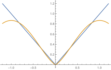
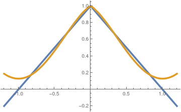
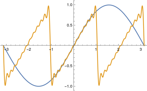
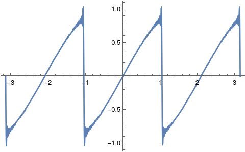
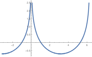
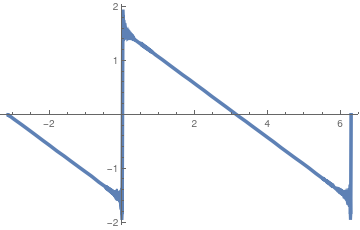
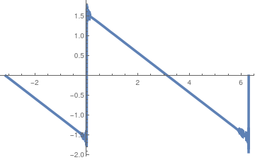
Let us consider two functions that can be used to generate saw-tooth graphs. One of them is the absolute value function (on a finite interval) and another one is just its shift:

\[ |x| \qquad \mbox{and} \qquad f(x) = \begin{cases} \ell -x, & \ \mbox{for} \quad 0 \le x < \ell , \\ \ell + x , & \ \mbox{for} \quad -\ell < x \le 0. \end{cases} \]
Using Mathematica, we find Fourier coefficients for the absolute value function.
Assuming[L > 0, Integrate[Abs[x]*Cos[n*Pi*x/L], {x, -L, L}]]
(2 L^2 (-1 + Cos[n \[Pi]] + n \[Pi] Sin[n \[Pi]]))/(n^2 \[Pi]^2)
Assuming[L > 0, Integrate[Abs[x], {x, -L, L}]]
L^2
\[ a_n (|x|) = \frac{1}{\ell} \int_{-\ell}^{\ell} |x|\,\cos \left( \frac{n\pi x}{\ell} \right) {\text d} x = \frac{2\ell}{n^2 \pi^2} \left( (-1)^n -1 \right) = - \frac{4\ell}{(2k-1)^2 \pi^2} , \qquad n=2k-1. \]
Then we use another command
Assuming[L > 0, FourierTrigSeries[Abs[x], x, 5, FourierParameters -> {1, Pi/L}]]
Therefore we get its Fourier series:
\[ |x| = \frac{\ell}{2} - \frac{4\ell}{\pi^2} \sum_{k\ge 1} \frac{1}{(2k-1)^2}\,\cos \left( \frac{\pi \left( 2k-1 \right) x}{\ell} \right) . \]
      We plot with Mathematica:
s20[x_] = 1/2 - (4/Pi^2)*Sum[Cos[k*Pi*x]/(2*k - 1)^2, {k, 1, 20}];
Plot[{Abs[x], s20[x]}, {x, -1.2, 1.2}, PlotStyle -> Thick]
       Absolute value function and its 20 term Fourier approximation.            Mathematica code

Now we calculate Fourier coefficients for function f(x)

Assuming[L > 0, Integrate[(L - x)*Cos[n*Pi*x/L], {x, 0, L}]/L] + Assuming[L > 0, Integrate[(L + x)*Cos[n*Pi*x/L], {x, -L, 0}]/L]
-((2 L (-1 + Cos[n \[Pi]]))/(n^2 \[Pi]^2))
This allows us to build the corresponding Fourier series
\[ f(x) = \frac{\ell}{2} + \frac{4\ell}{\pi^2} \sum_{k\ge 1} \frac{1}{(2k-1)^2}\,\cos \left( \frac{\pi \left( 2k-1 \right) x}{\ell} \right) . \]
      We plot with Mathematica:
s20[x_] = 1/2 + (4/Pi^2)*Sum[Cos[k*Pi*x]/(2*k - 1)^2, {k, 1, 20}];
f[x_] = Piecewise[{{1 + x, x < 0}, {1 - x, x > 0}}];
Plot[{f[x], s20[x]}, {x, -1.2, 1.2}, PlotStyle -> Thickness[0.01]]
       Function f(x) and its 20 term Fourier approximation.            Mathematica code

      We plot with Mathematica 50 term approximation to its conjugate Fourier series (which is very close to sine function):
\[ S^{\ast} [f](x) = \frac{4\ell}{\pi^2} \sum_{k\ge 1} \frac{1}{(2k-1)^2}\,\sin \left( \frac{\pi \left( 2k-1 \right) x}{\ell} \right) . \]
s50[x_] = (4/Pi^2)*Sum[Sin[k*Pi*x]/(2*k - 1)^2, {k, 1, 50}];
Plot[{(4/Pi^2)*Sin[Pi*x], s50[x]}, {x, -1.2, 1.2}, PlotStyle -> Thickness[0.01]]
       Function f(x) and its 20 term Fourier approximation.            Mathematica code

End of Example 2

A derivation of Euler--Fourier formulas \eqref{EqFourier.2} and \eqref{EqFourier.4} are given in section devoted to orthogonal expansions.

The complex Fourier series \eqref{EqFourier.1} is more elegant and shorter to write down than the one expressed in terms of sines and cosines \eqref{EqFourier.3}, but it has the disadvantage that the coefficients might be complex numbers even if the given function is real-valued. The trigonometric form is based on Euler's formulas:

\[ \sin \theta = \frac{1}{2{\bf j}} \,e^{{\bf j}\theta} - \frac{1}{2{\bf j}} \,e^{-{\bf j}\theta} = \Im \,e^{{\bf j}\theta} = \mbox{Im} \,e^{{\bf j}\theta}, \qquad \cos \theta = \frac{1}{2} \,e^{{\bf j}\theta} + \frac{1}{2} \,e^{-{\bf j}\theta} = \Re \,e^{{\bf j}\theta} = \mbox{Re} \,e^{{\bf j}\theta}. \]

Here, j is the unit vector in the positive vertical direction on the complex plane ℂ, so j² = −1. Of course, these two decompositions \eqref{EqFourier.1} and \eqref{EqFourier.3} are equivalent when each series \eqref{EqFourier.1} and \eqref{EqFourier.3} converges.

In a memorable session of the French Academy on the 21st of December 1807, the mathematician and politician Joseph Fourier announced a thesis that commenced a new chapter in mathematical physics. The claim of Fourier appeared to the older members of the Academy, including the great analyst Lagrange, as entirely incredible. Fourier claimed that an arbitrary function, defined in a finite interval by an arbitrarily capricious graph, can always be decomposed into a sum of pure sine and cosine functions. The academicians had good reasons to question Fourier's theorem. Any superposition of sine and cosine functions could never give anything but an infinitely differentiable function called holomorphic or analytic. Such a function was very far from the capricious course of an arbitrarily drawn graph. In fact, an analytic function had the property" that given its course in an arbitrarily small interval, the continuation of its course to the right and to the left was uniquely determined. How could one reconcile this fact with the generality claimed by Fourier's theorem?

Subsequent investigations demonstrated that Fourier's claim was entirely justified, although he himself was not able to provide the exact proofs demanded, because the corresponding theory, called after Sturm (1803--1855) and Liouville (1809--1882) appeared only thirty years later.

Fourier dissertation (and successive monograph publication in 1822) initiated further development in mathematics. First of all, the cornerstone concept of function was establish. Before Fourier's discovery, functions were considered either by analytic formula or geometrically if they could be drawn with the hand. Daniel Bernoulli (1700--1782) believed that any functions can be defined by a formula.

In the later development of mathematics, evaluation of Fourier coefficients requres a proper definition of integrability that was successfully addressed by Bernhard Riemann (1826--1866). He developed a concept of " Riemann-integrability" in 1854, but not published in a journal until 1868. Even this definition was not sufficient for the more abstract speculations of modern mathematics and was once more generalized by Émile Borel (1871--1956) and Henri Lebesgue (1875--1941), who in 1904 extending the applicability of the Fourier series to a still larger class of functions.

Note that for all applications of the Fourier series in relation to the physical universe the less sophisticated concept of Riemann is quite satisfactory.

It is well-known that partial Fourier sums display in general a rather irregular behavior as the number of terms grows to infinity. In 1900, Lipót Fejér discovered that the Cesàro means (which is an extension of regular summation method) of the partial sums display a strikingly simpler behavior. This broadened the validity of the Fourier series to a much larger class of functions that does not demand more than mere integrability of functions, without adding any other restrictions concerning continuity or differentiability.

In 1902, Jacques Salomon Hadamard (1865--1963) introduced definition of well-posed problem. Correspondingly, a problem that is not well-posed, is called ill-posed. It turns out that restoration of a function from its set of Fourier coefficients is an ill-posed problem. This becomes clear in 1899 when Willard Gibbs reported a phenomenon of conditionally convergent Fourier series that now bare his name. Actually, it was known 50 years before to Henry Wilbraham (1825--1883).
﹡ ⁎ ✱ ✲ ✳ ✺ ✻ ✼ ✽ ❋ <


Finite Partial Sums of Fourier Series


For any real x, the finite sum
\[ F_N (x) = \frac{a_0}{2} + \sum_{k=1}^{N} \left[ a_k \cos \left( \frac{k \pi x}{\ell} \right) + b_k \sin \left( \frac{k \pi x}{\ell} \right) \right] \]
or
\[ F_N (x) = \sum_{k=-N}^{N} \alpha_n e^{{\bf j}n \pi x/\ell} \]
is called a trigonometric polynomial of order N.

In calculus, you learnt that an infinite series \( \sum_{k\ge 0} a_k \) converges (or is convergent) to S if the sequence of partial sums \( S_n = \sum_{k= 0}^n a_k \) tends to S as n → ∞. In case of Fourier series, elements of series depend on real parameter x ∈ [−ℓ, ℓ], and we come to definition of its partial sums.

Theorem 1: For any real-valued function f : [−ℓ, ℓ] → ℝ and any positive integer N ∈ ℕ = { 0, 1, 2, … }, its N-th partial Fourier exponential sum
\begin{equation} \label{EqFourier.5} S_N (f;x) = \sum_{n=-N}^N \hat{f}(n)\,e^{{\bf j} n\pi x/\ell} \end{equation}
and N-th partial Fourier trigonometric sum
\begin{equation} \label{EqFourier.6} S_N (f;x) = \frac{1}{2}\,a_0 + \sum_{k=1}^N \left[ a_k \cos \left( \frac{k\pi x}{\ell} \right) + b_k \sin \left( \frac{k\pi x}{\ell} \right) \right] \end{equation}
are the same; here coefficients 𝑎k, bk and \( \displaystyle \hat{f}(n) \) are determined by the Euler--Fouier formulas \eqref{EqFourier.2} and \eqref{EqFourier.4}, respectively. Moreover, the N-th partial Fourier sum is expressed in an integral form, known as a convolution, which is denoted by star:
\[ S_N (f;x) = \frac{1}{\ell} \int_{-\ell}^{\ell} f(y)\,D_N \left( \frac{\pi (x-y)}{\ell} \right) {\text d}y = \frac{1}{\ell} \left( f \star D_N \right) (x), \]
where DN(z) is called the Dirichlet kernel, and
\[ D_N (z) = \frac{\sin \left( N + \frac{1}{2} \right) z}{2\,\sin\frac{z}{2}} . \]
Note that according to the L'Hôpital's rule, DN(0) = N + ½. It is a custom to utilize ★ for convolution of two functions:
\[ \left( f \star g \right) (x) = g \star f (x) = \int f(y) g(x-y)\,{\text d} y . \]
We are going to prove the statement for a particular case when ℓ = π in order to simplify calculations. We compute
\begin{align*} S_N (f; x) &= \sum_{n=-N}^N \hat{f}(n) \,e^{{\bf j}nx} = \sum_{n=-N}^N \frac{1}{2\pi} \int_{-\pi}^{\pi} f(y)\,e^{-{\bf j}n y} {\text d}y\, e^{{\bf j}nx} \\ &= \frac{1}{2\pi} \int_{-\pi}^{\pi} f(y) \sum_{n=-N}^N e^{{\bf j}n\left( x-y \right)} \\ &= \frac{1}{\pi} \int_{-\pi}^{\pi} f(y)\,D_N (x-y) \,{\text d}y = \frac{1}{\pi} \, f \star D_N (x) . \end{align*}
Here
\[ D_N (t) = \frac{1}{2}\,\delta_N (t) = \frac{1}{2} \sum_{n=-N}^N e^{{\bf j}n t} \qquad ({\bf j}^2 =1) \]
is the Dirichlet kernel. Also, fg means the convolution of f and g, which is defined as
\[ f \star g (x) = \int_{-\ell}^{\ell} f(y)\,g(x-y)\,{\text d}y = \int_{-\ell}^{\ell} f(x-y)\,g(y)\,{\text d}y = g \star f . \]
Next, we have
\begin{align*} \delta_N (x) &= \sum_{n=-N}^N e^{{\bf j} n x} = e^{-{\bf j} N x} \sum_{n=0}^{2N} e^{{\bf j} n x} \\ &= e^{-{\bf j} N x} \frac{1 - e^{-{\bf j} \left( 2N+1 \right) x}}{1 - e^{{\bf j} x}} = \frac{e^{-{\bf j} Nx} - e^{-{\bf j} \left( N+1 \right) x}}{1 - e^{{\bf j} x}} \\ &= \frac{e^{-{\bf j} \left( N + \frac{1}{2} \right) x} - e^{{\bf j} \left( N + \frac{1}{2} \right) x}}{e^{-{\bf j} x/2} - e^{-{\bf j} x/2}} \\ &= \frac{\sin \left( N + \frac{1}{2} \right) x}{\sin\frac{x}{2}} \end{align*}
because
\[ \sin\theta - \frac{1}{2{\bf j}} \left( e^{{\bf j}\theta} - e^{-{\bf j}\theta} \right) . \]


The formula for trigonometric partial sum is proved in Lemma 1 of convergence section.
Lemma 1: The following integrals diverge:
\[ \lim_{N\to\infty}\int_{-\pi}^{\pi} D_N (x)^2 {\text d} x = \infty , \qquad \mbox{and} \qquad \int_{-\pi}^{\pi} \left\vert D_N (x) \right\vert {\text d} x \ge 4\,\mbox{Si}(\pi ) + \frac{8}{\pi}\,\ln n , \]
where Si(x) is the sine integral.
For any small δ, we break the integral into three parts:
\[ I_N = \int_{-\pi}^{\pi} D_N (x)^2 {\text d} x = I_{\delta} (N) + I_2 + I_3 , \]
where
\[ I_{\delta} (N) = 8 \int_{0}^{\delta} \frac{\sin^2 \left( N + \frac{1}{2} \right) x}{x^2} \, {\text d} x , \]
and
\[ I_2 = \int_{|x| \le \delta} \sin^2 \left( N + \frac{1}{2} \right) x \left( \frac{1}{\sin^2 \frac{x}{2}} - \frac{4}{x^2} \right) {\text d} x , \qquad I_3 = \int_{|x| > \delta} D_N (x)^2 {\text d} x . \]
Since the kernel of integral I2 is bounded in a neighborhood of the origin,
Series[1/(Sin[x/2])^2 - 4/x^2, {x, 0, 5}]
SeriesData[x, 0, { Rational[1, 3], 0, Rational[1, 60], 0, Rational[1, 1512]}, 0, 6, 1]
both integrals, I2 and I3, tend to zero as N → ∞ according to Riemann--Lebesgue lemma. Using substitution s = (N + ½)x in integral Iδ, we get
\[ I_{\delta} (N) = 4 \left( 2N + 1 \right) \int_{0}^{\delta \left( N + 1/2\right)} \frac{\sin^2 s}{s^2}\, {\text d}s . \]
Since the latter integral converges
Integrate[(Sin[s])^2/s^2, {s, 0, Infinity}]
\[Pi]/2
\[ \int_0^{\infty} \frac{\sin^2 s}{s^2}\,{\text d}s = \frac{\pi}{2} , \]
we conclude that
\[ I_{\delta} (N) = O\left( 2N + 1 \right) \to \infty \qquad\mbox{as} \quad s N \to infty . \]
End of Proof for the first part
We have
\begin{align*} \| D_N (x) \|_1 &= \int_{-\pi}^{\pi} \left\vert D_N (x) \right\vert {\text d}x = 2 \int_{0}^{\pi} \left\vert D_N (x) \right\vert {\text d}x \ge \int_0^{\pi} \frac{\left\vert \sin [(2N+1) x/2] \right\vert}{x}\,{\text d} x \end{align*}
because \( \displaystyle \frac{2}{x} \le \frac{1}{\left\vert \sin (x/2) \right\vert} . \) In the latter integral, we make substitution \( \displaystyle t = \left( 2N+1 \right) x/2 \) to obtain
\begin{align*} \| D_N (x) \|_1 &\ge \int_0^{(2N+1) \pi /2} \frac{|\sin t|}{t}\,{\text d}t \\ &= \sum_{k=0}^{N-1} \int_{k\pi}^{(k+1)\pi} \frac{|\sin t|}{t}\,{\text d}t + \int_{N\pi}^{N\pi + \pi /2}\frac{|\sin t|}{t}\,{\text d}t \\ &\ge \sum_{k=0}^{N-1} \int_{k\pi}^{(k+1)\pi} \frac{|\sin t|}{(k+1)\pi}\,{\text d}t + \int_{N\pi}^{N\pi + \pi /2}\frac{|\sin t|}{\pi \left( N + 1/2 \right)}\,{\text d}t . \end{align*}
In each integral of the latter sum, we change the dummy variable of integration so each integration starts from zero:
\begin{align*} \| D_N (x) \|_1 &\ge \left\vert \sum_{k=0}^{N-1} \int_0^{\pi} \frac{\sin (s)} {\left( k+1 \right) \pi} \,{\text d} s \right\vert + \frac{1}{\left( N + 1/2 \right) \pi} \int_0^{\pi /2} \frac{\sin (s)}{s} \,{\text d} s \\ & \ge \frac{2}{\pi} \sum_{k=0}^{N-1} \frac{1}{k+1} + \frac{2}{\left( 2N + 1 \right) \pi} \,\mbox{Si} \left( \frac{\pi}{2} \right) \\ &= \frac{2}{\pi}\, H_N + \frac{2}{\left( 2N + 1 \right) \pi} \,\mbox{Si} \left( \frac{\pi}{2} \right) , \end{align*}
where HN is the harmonic number that approaches infinity as logarithm when N → ∞. Indeed, Hn = lnn + γ +o(n) as n → ∞, where γ = 0.5772156649 is the Euler–Mascheroni constant.
The Dirichlet kernel is related to Fourier expansion of the Dirac delta function:
\[ \delta (x-a) = \frac{1}{2\pi} \, \int_{-\infty}^{\infty} e^{{\bf j} (x-a)t} \, {\text d} t = \lim_{n\to \infty} \, \frac{1}{2\pi} \, \sum_{k=-n}^n \, e^{{\bf j} k(x-a)} \quad \left( = \frac{\sin \left[ \left( n+ \frac{1}{2} \right) (x-a) \right]}{2\pi\, \sin \frac{x-a}{2}} \right) , \]
where j is the unit vector in the positive vertical direction on the complex plane ℂ, so j² = −1.

Example 3: The following sum

\[ D_N^{\ast} = \sum_{k=1}^N \sin (kx) = \frac{\cos \frac{x}{2} - \cos \left( N + \frac{1}{2} \right) x}{2\,\sin\frac{x}{2}} \tag{3.1} \]
is known as the Dirichlet conjugate kernel. The derivation of formula (3.1) is based on extracting the imaginary part of
\[ \sum_{k=1}^N z^k = \Im \frac{z - z^{N+1}}{1-z} , \qquad z = e^{{\bf j} x} . \]
Multiplying by the complex conjugate (1 - z)*, we get
\[ D_N^{\ast} = \Im \frac{z - z^{N+1}}{1-z} \cdot \frac{(1-z)^{\ast}}{( 1- z)^{\ast}} = \Im \frac{z - z^{N+1} -|z|^2 - z^{N+1} z^{\ast}}{(1-\cos x)^2 + \sin^2 x} . \tag{3.2} \]
Extraction of the imaginary part yields
\[ D_N^{\ast} = \frac{\sin x - \sin (N+1) x - \sin Nx}{2 - 2\,\cos x} \]
Then using trigonometric identities
\begin{align*} 2\,\sin\alpha\,\cos\beta &= \sin \left( \alpha + \beta \right) + \sin \left( \alpha - \beta \right) , \qquad \alpha = 1/2, \quad \beta = N + 1/2 , \\ \sin x &= 2 \sin\tfrac{x}{2}\,\cos \tfrac{x}{2} , \\ 1- \cos x &= 2\,\sin^2 \tfrac{x}{2} , \end{align*}
we derive the required formula for the Dirichlet conjugate kernel. ■


Change of Scale


Coefficient evaluations in the Euler--Fourier formulas \eqref{EqFourier.2} and \eqref{EqFourier.4} can be obtained upon integration over any interval of length T = 2ℓ because of periodically condition. Sometimes it is convenient to consider a function on interval [0,T] (or any interval of length T). Let f(x) be a periodic function over the range 0 ≤ x < T. Then its Fourier series becomes
\[ f(x) \,\sim\, \frac{a_0}{2} + \sum_{k\ge 1} \left[ a_k \cos \left( \frac{2k \pi x}{T} \right) + b_k \sin \left( \frac{2k \pi x}{T} \right) \right] , \tag{4} \]
where coefficients are defined as
\[ \left[ \begin{array}{c} a_k \\ b_k \end{array} \right] = \frac{2}{T} \int_{0}^{T} f(x) \left[ \begin{array}{c} \cos \left( \frac{2\pi kx}{T} \right) \\ \sin \left( \frac{2\pi kx}{T} \right) \end{array} \right] {\text d} x , \qquad k= 0, 1, 2, 3, \ldots . \tag{5} \]
A similar expression is valid for exponential Fourier series.

In general, a square integrable function f ∈ 𝔏²([𝑎, b]) on the interval [𝑎, b] of positive length b−𝑎 (b>𝑎) can be expanded into the Fourier series

\begin{equation} \label{EqFourier.7} f(x) \,\sim\, \frac{a_0}{2} + \sum_{k=1}^{\infty} \left[ a_k \cos \left( \frac{2\pi k (x - a)}{b-a} \right) + b_k \sin \left( \frac{2\pi k (x - a)}{b-a} \right) \right] , \end{equation}
where
\begin{align} a_k &= \frac{2}{b-a} \int_a^b f(x) \,\cos \left( \frac{2\pi k(x - a)}{b-a} \right) {\text d}x , \qquad k=0,1,2,\ldots , \notag \\ \label{EqFourier.8} \\ b_k &= \frac{2}{b-a} \int_a^b f(x) \,\sin \left( \frac{2\pi k(x - a)}{b-a} \right) {\text d}x , \qquad k=1,2,\ldots . \notag \end{align}

Example 4: Consider a function f(x) = x² on the interval [0,2]. Its Fourier coefficients can be determined with Mathematica:

Integrate[x^2, {x, 0, 2}]
8/3
Simplify[Integrate[x^2 * Cos[n*Pi*x], {x, 0, 2}], Assumptions -> Element[n, Integers]]
4/(n^2 \[Pi]^2)
Simplify[Integrate[x^2 * Sin[n*Pi*x], {x, 0, 2}], Assumptions -> Element[n, Integers]]
4/(n \[Pi])
Therefore, we get the following Fourier series for function x²:
\[ x^2 = \frac{4}{3} + \sum_{n\ge 1} \left[ \frac{4}{n^2 \pi^2}\,\cos \left( n\pi x \right) - \frac{4}{n\,\pi}\,\sin \left( n\pi x \right) \right] . \]
Next we plot some partial sums along with the given function x²
S10[x_] = 4/3 + Sum[4/n^2/Pi^2 *Cos[n*Pi*x] - 4/n/Pi*Sin[n*Pi*x], {n, 1, 10}];
S20[x_] = 4/3 + Sum[4/n^2/Pi^2 *Cos[n*Pi*x] - 4/n/Pi*Sin[n*Pi*x], {n, 1, 20}];
S100[x_] = 4/3 + Sum[ 4/n^2/Pi^2 *Cos[n*Pi*x] - 4/n/Pi*Sin[n*Pi*x], {n, 1, 100}];
Plot[{x^2, S10[x]}, {x, -0.5, 2.5}, PlotStyle -> {Thick, {Black, Red}}]
Plot[{x^2, S20[x]}, {x, -0.5, 2.5}, PlotStyle -> {Thick, {Black, Orange}}]
Plot[{x^2, S100[x]}, {x, -0.5, 2.5}, PlotStyle -> {Thick, {Black, Blue}}]
   Fourier approximation with 10 terms    Fourier approximation with 20 terms    Fourier approximation with 100 terms
       

Now we expand the given function f(x) = x² into complex Fourier series \eqref{EqFourier.1}:

\[ x^2 = \frac{4}{3} + \mbox{P.V.}\,\sum_{n\ne 0} \left( \frac{2}{n^2 \pi^2} + \frac{2{\bf j}}{n\pi} \right) e^{n{\bf j}\pi x} . \]
Integrate[x^2 *Exp[-n*I*Pi*x], {x, 0, 2}]/2
(E^(-2 I n \[Pi]) (-2 I + 2 I E^(2 I n \[Pi]) + 4 n \[Pi] + 4 I n^2 \[Pi]^2))/(2 n^3 \[Pi]^3)
Integrate[x^2 *Exp[-0*I*Pi*x], {x, 0, 2}]/2
4/3

Example 5: 
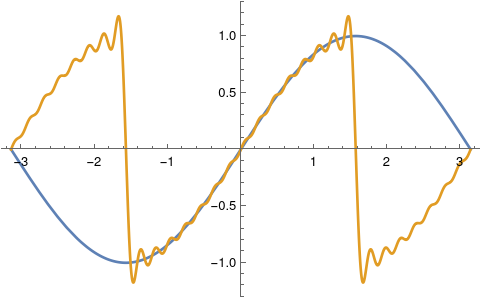
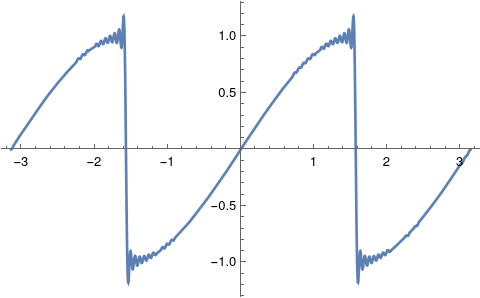
We expand the sine function into Fourier series for different values of parameter ℓ that defines the interval from which a function is periodically expanded.

Example 5A: Let us start with ℓ = π. Then sinx itself is its Fourier series; so no work is required.

Example 4B: For ℓ = π/2, we get Fourier coefficients

\[ \hat{f} (n) = \frac{1}{\pi} \int_{-\pi /2}^{\pi /2} \sin x\, e^{-n{\bf j}2x} {\text d}x = \frac{4n{\bf j}}{\left( 4n^2 -1 \right) \pi} \left( -1 \right)^n , \qquad n = 0, \pm 1, \pm2 , \ldots . \]
Integrate[Sin[x]*Exp[-n*I*2*x], {x, -Pi/2, Pi/2}]/Pi
(4 I n Cos[n \[Pi]])/((-1 + 4 n^2) \[Pi])
This provides the exponential Fourier series of sine function:
\[ \sin x = \mbox{P.V.} \frac{1}{\pi} \sum_{n=-\infty}^{\infty} \frac{4n{\bf j}}{4n^2 -1} \left( -1 \right)^n e^{{\bf j}2nx} . \]
Fourier coefficients for trigonometric series are
\[ a_k = \frac{2}{\pi} \int_{-\pi /2}^{\pi /2} \sin x\, \cos \left( 2k x \right) {\text d} x = 0 0 \]
and
\[ b_k = \frac{2}{\pi} \int_{-\pi /2}^{\pi /2} \sin x\, \sin \left( 2k x \right) {\text d} x = \frac{8k}{\left( 1 - 4k^2 \right) \pi} \, (-1)^k . \]
We plot the corresponding approximations with 15 and 50 term.
S15[x_] = (8/Pi)*Sum[n/(1 - 4*n^2 )*(-1)^n * Sin[2*n*x], {n, 1, 15}];
Plot[{Sin[x], S15[x]}, {x, -Pi, Pi}, PlotStyle -> Thick]
S50[x_] = (8/Pi)*Sum[n/(1 - 4*n^2 )*(-1)^n * Sin[2*n*x], {n, 1, 50}];
Plot[{S50[x]}, {x, -Pi, Pi}, PlotStyle -> Thick]
   Fourier approximation with 15 terms           Fourier approximation with 50 terms
          

Example 5C: For ℓ = π/3, we get Fourier coefficients

\[ \hat{f} (n) = \frac{3}{2\pi} \int_{-\pi /3}^{\pi /3} \sin x\, e^{-n{\bf j}3x} {\text d}x = \frac{9\sqrt{3}n{\bf j}}{\left( 9n^2 -1 \right) 2\pi} \left( -1 \right)^n , \qquad n = 0, \pm 1, \pm2 , \ldots . \]
Integrate[Sin[x]*Exp[-n*I*3*x], {x, -Pi/3, Pi/3}]*(3/2/Pi)
(3 I (3 Sqrt[3] n Cos[n \[Pi]] - Sin[n \[Pi]]))/(2 (-1 + 9 n^2) \[Pi])
This provides the exponential Fourier series of sine function on interval (−π/3, π/3):
\[ \sin x = \frac{9\sqrt{3}}{2\pi} \sum_{n=-\infty}^{\infty} \frac{n{\bf j}}{9n^2 -1} \left( -1 \right)^n e^{{\bf j}3nx} . \]
Fourier coefficients for trigonometric series are
\[ a_k = \frac{3}{\pi} \int_{-\pi /3}^{\pi /3} \sin x\, \cos \left( 3k x \right) {\text d} x = \]
and
\[ b_k = \frac{3}{\pi} \int_{-\pi /3}^{\pi /3} \sin x\, \sin \left( 3k x \right) {\text d} x = -\frac{9\sqrt{3}\,k}{\left( 9 \k^2 -1 \right) \pi} \left( -1 \right)^k , \qquad k=1,2,3,\ldots . \]
Integrate[Sin[x]*Cos[k*3*x], {x, -Pi/3, Pi/3}]*(3/Pi)
0
Integrate[Sin[x]*Sin[k*3*x], {x, -Pi/3, Pi/3}]*(3/Pi)
(3 (-3 Sqrt[3] k Cos[k \[Pi]] + Sin[k \[Pi]]))/((-1 + 9 k^2) \[Pi])
We plot the corresponding approximations with 12 and 55 term.
S12[x_] = (9*Sqrt[3]/Pi)* Sum[n/(1 - 9*n^2)*(-1)^n*Sin[3*n*x], {n, 1, 12}];
Plot[{Sin[x], S12[x]}, {x, -Pi, Pi}, PlotStyle -> Thick]
S55[x_] = (9*Sqrt[3]/Pi)* Sum[n/(1 - 9*n^2)*(-1)^n*Sin[3*n*x], {n, 1, 55}];
Plot[{S55[x]}, {x, -Pi, Pi}, PlotStyle -> Thick]
   Fourier approximation with 12 terms           Fourier approximation with 55 terms


Evaluation of Fourier Coefficients


Numerical evaluation of Fourier coefficients becomes a challenging problem for large indices because it leads to integrals with very fast oscillating integrands.

The following formulas could be helpful for evaluations of Fourier coefficients (\( \texttt{D} = \texttt{D}_t = {\text d}/{\text d}t \) is the derivative operator):
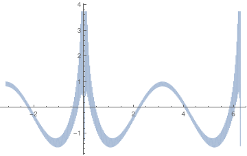
Theorem 2:
\begin{align*} \int t^n \cos (at) \,{\text d}t &= - \frac{1}{a} \sum_{k=0}^n \frac{1}{a^k} \, {\texttt D}_t^k \left( t^k \right) \left. {\texttt D}_z^{k+1} \left( \cos z \right) \right\vert_{z=at} \\ &= - \frac{1}{a} \left[ t^n {\texttt D}_z \cos z + \frac{n\,t^{n-1}}{a} \, {\texttt D}_z^2 \cos z + \cdots + \frac{n!}{a^n} \, {\texttt D}_z^{n+1} \cos z \right]_{z=at} , \\ \int t^n \sin (at) \,{\text d}t &= - \frac{1}{a} \sum_{k=0}^n \frac{1}{a^k} \, {\texttt D}_t^k \left( t^k \right) \left. {\texttt D}_z^{k+1} \left( \sin z \right) \right\vert_{z=at} \\ &= - \frac{1}{a} \left[ t^n {\texttt D}_z \sin z + \frac{n\,t^{n-1}}{a} \, {\texttt D}_z^2 \sin z + \cdots + \frac{n!}{a^n} \, {\texttt D}_z^{n+1} \sin z \right]_{z=at} .     \end{align*}

Example 15: 
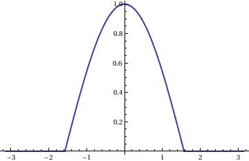
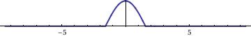
Let's consider the following half-wave rectifier of the function cosx on interval [−π/2, ;π/2]:

\[ f(x) = \begin{cases} \cos x, & \ \mbox{ when } \ -\frac{\pi}{2} \le x \le \frac{\pi}{2} , \\ 0 , & \ \mbox{ when } \ \frac{\pi}{2} \le x \le \frac{3\pi}{2} . \end{cases} \]
Outside the interval of length 2π, the function f(x) is expanded periodically.
f[t_] = Piecewise[{{Cos[t], -Pi/2 < t < Pi/2}, {0, -Pi < t < -Pi/2 && Pi/2 < t < Pi}}]
Out[1]= { Cos[t] - Pi/2 < t < Pi/2
             { 0 True
Plot[f[t], {t, -Pi, Pi}, PlotStyle -> Thick]

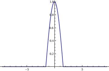
Mathematica will treat the function f[t] outside the interval [-π , π ] as zero

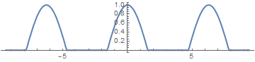
Plot[f[t], {t, -3*Pi, 3*Pi}, PlotStyle -> Thick]

As we see, Mathematica rescales vertical and horizontal lines so that the picture becomes almost symmetric. You can return to the proper picture by using AspectRatio option:

Plot[f[t], {t, -3*Pi, 3*Pi}, PlotStyle -> Thick, AspectRatio -> 1/3/Pi, Ticks -> {True, None}]

So we get exactly the same graph. Now we are ready to expand this function into Fourier series by finding its Fourier coefficients:

\begin{align*} a_0 &= \frac{1}{\pi} \int_{-\pi /2}^{\pi /2} \cos x\,{\text d} x = \frac{2}{\pi} , \\ a_k &= \frac{1}{\pi} \int_{-\pi /2}^{\pi /2} \cos x\, \cos \left( k\, x \right) {\text d} x = -\frac{2}{\pi}\, \frac{1}{k^2 -1} \, \cos \frac{k\pi}{2} , \qquad k= 2, 3, \ldots ; \\ b_k &= \frac{1}{\pi} \int_{-\pi /2}^{\pi /2} \cos x\, \sin \left( k\, x \right) {\text d} x =0, \qquad k= 1, 2, 3, \ldots . \end{align*}
Then the corresponding Fourier series becomes
\[ f(t) \,=\,\frac{1}{\pi} + \frac{1}{2}\, \cos t - \frac{2}{\pi} \, \sum_{k\ge 1} \frac{1}{k^2 -1} \,\cos \left( k\, x \right) . \]
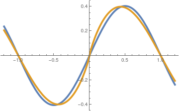
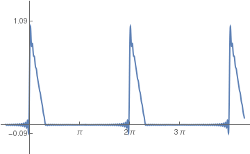
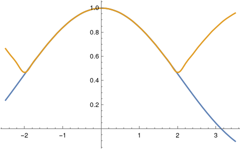
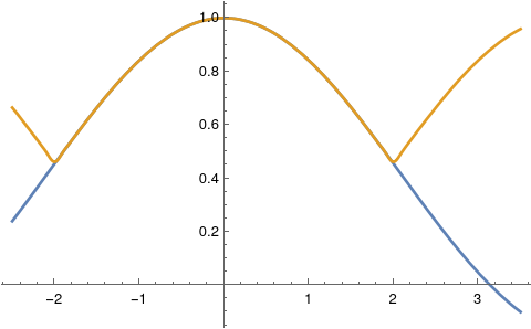
A partial sum with N = 20 terms gives a very good approximation:

Example 16: 
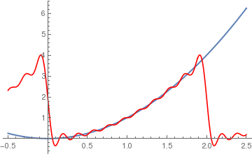
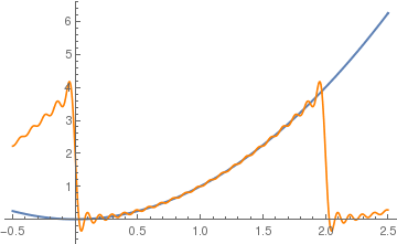
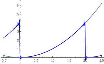
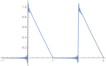
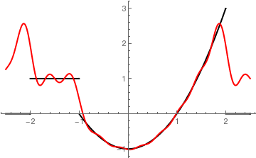
We consider a piecewise continuous function that cannot be extended into Taylor series because it is identically zero on the interval (1,2). However, we can find its Fourier series.

f[x_] = Piecewise[{{1 - x, 0 < x < 1}, {0, 1 < x < 2}}]
Out[2]= { 1-x, if 0<x<1 and 0 for 1<x<2.

The standard Mathematica command FourierTrigSeries provides you the Fourier series of the function that is extended periodically from the standard interval (-π,π):

FourierTrigSeries[f[x], x, 3]
Out[2]= 1/(4 \[Pi]) + (2 Cos[x] Sin[1/2]^2)/\[Pi] + (Cos[2 x] Sin[1]^2)/(2 \[Pi]) + (2 Cos[3 x] Sin[3/2]^2)/(
9 \[Pi]) + ((2 - 2 Sin[1]) Sin[x])/(2 \[Pi]) - ((-2 + Sin[2]) Sin[2 x])/(4 \[Pi]) - ((-3 + Sin[3]) Sin[3 x])/(9 \[Pi])

With option FourierParameters, it is equivalent to

FourierTrigSeries[f[x], x, 3, FourierParameters -> {1, 1}]
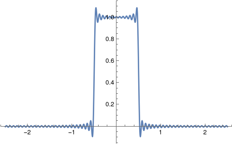
We can plot the partial sum with say 50 terms. Since Fourier partial sums oscillate near points of discontinuity exhibiting so called Gibbs phenomenon, we indicate maximum wiggle (overshoot) and minimum one:

curve = FourierTrigSeries[f[x], x, 50];
Plot[curve, {x, -1.5, 13.5}, PlotRange -> {-0.3, 1.3}, Ticks -> {{Pi, 2*Pi, 3*Pi}, {1.09, -0.09}}, PlotStyle -> Thick]

However, it is not what we want: we need the Fourier series of the function f[x] extended periodically from the interval of length 2:

FourierTrigSeries[f[x], x, 3, FourierParameters -> {1, Pi}]
Out[3]= 1/4 + (2 Cos[\[Pi] x])/\[Pi]^2 + (2 Cos[3 \[Pi] x])/(9 \[Pi]^2) + Sin[\[Pi] x]/\[Pi] + Sin[2 \[Pi] x]/(2 \[Pi]) + Sin[3 \[Pi] x]/( 3 \[Pi])

To check, we find the Fourier coefficients manually:

Integrate[f[x]*Cos[n*Pi*x], {x, 0, 2}, Assumptions -> Element[n, Integers]]
Out[4]= (1 - Cos[n \[Pi]])/(n^2 \[Pi]^2)
So
\[ a_0 = \frac{1}{2} , \qquad a_n = \frac{1- (-1)^n}{n^2 \pi^2} , \quad n=1,2,\ldots . \]
Integrate[f[x]*Sin[n*Pi*x], {x, 0, 2}, Assumptions -> Element[n, Integers]]
Out[5]= (n \[Pi] - Sin[n \[Pi]])/(n^2 \[Pi]^2)

which is 1/(n*π). Hence, its Fourier series becomes

\[ f(x) = \frac{1}{4} + \sum_{n\ge 1} \left[ \frac{1- (-1)^n}{n^2 \pi^2} \, \cos \left( n \pi x \right) + \frac{1}{n\pi}\, \sin \left( n \pi x \right) \right] \]
We can also represent f(x) in other forms:
\[ f(x) = \frac{1}{4} + \sum_{n\ge 1} \sqrt{ \left( \frac{1- (-1)^n}{n^2 \pi^2} \right)^2 + \frac{1}{n^2 \pi^2}} \, \sin \left( n \pi x + \arctan \frac{1- (-1)^n}{n \pi} \right) = \frac{1}{4} + \sum_{n\ge 1} \sqrt{ \left( \frac{1- (-1)^n}{n^2 \pi^2} \right)^2 + \frac{1}{n^2 \pi^2}} \, \cos \left( n \pi x - \mbox{arccot} \frac{1- (-1)^n}{n \pi} \right) . \]
Now we plot some partial sums, starting with the given function itself:

Plot[f[x], {x, -1, 3}, PlotRange -> {0, 1}, AspectRatio -> Automatic, Axes -> {True, False}, PlotStyle -> Thick]

Then we plot some finite sums:

curve5Pi = FourierTrigSeries[f[x], x, 5];
Plot[%, {x, -1, 3}]

Then we repeat calculations with 50 terms:


Next we plot the correct Fourier series partial sums:

curve5=FourierTrigSeries[f[x], x, 50, FourierParameters -> {1, Pi}];
Plot[%, {x, -1, 3}]


There is an elegant application of Fourier series involving Bessel functions:
\[ \cos \left( a\,\sin x \right) = J_0 (a) + \sum_{k\ge 1} J_{2k} (a) \,\cos \left( 2kx \right) . \]

Computing an integral in Mathematica is fairly painless, and it's tempting to simply use a partial Fourier sum depending to the number of terms n. We show how these commands work with several examples.

Mathematica has four default commands to calculate Fourier series:

FourierSeries        (* to calculate complex coefficient expansion *)
FourierTrigSeries  (* to calculate standard Fourier expansion via sine and cosine *)
FourierCosSeries (* to calculate cosine Fourier series *)
FourierSinSeries   (* to calculate sine Fourier series *)


The option FourierParameters has two parameters and when applied, it looks as FourierParameters->{𝑎,b}
In trigonometric form, with setting \( {\bf FourierParameters} \,-> \,\{ a, b \} \) the following series is returned:

\[ \left\vert \frac{b}{\pi} \right\vert^{(1+a)/2} \left[ \frac{a_0}{2} + \sum_{k=1}^n \left( a_k \,\cos (bkt) + b_k \,\sin (bkt) \right) \right] , \]
with
\[ a_k = \left\vert \frac{b}{\pi} \right\vert^{(1+a)/2} \,\int_{-\pi/|b|}^{\pi/|b|} f(t)\,\cos (bkt) \,{\text d}t , \qquad k=0,1,2,\ldots , \]
\[ b_k = \left\vert \frac{b}{\pi} \right\vert^{(1+a)/2} \,\int_{-\pi/|b|}^{\pi/|b|} f(t)\,\sin (bkt) \,{\text d}t , \qquad k=1,2,\ldots . \]

Syntax for the FourierSeries command is: FourierSeries [ function , variable , number of terms ]

Changing the FourierParameters setting allows you to control the limits of integration on the coefficients, and therefore, the base frequency of the series. Some work will go into calculating what value for “b” will give the proper limits of integration. There is ordinarily no reason to change “𝑎” from its default setting, which is 1.
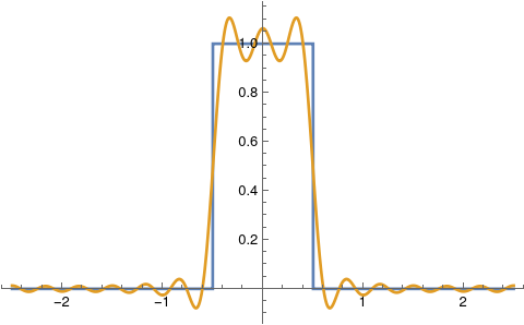
Example 6: We consider a pulse function of length h:
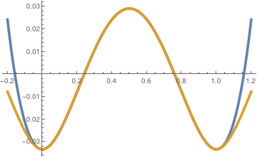
\[ f(x) = \begin{cases} 1 , & \quad\mbox{for} \quad -h/2 < x < h/2 , \\ 0, & \quad\mbox{otherwise}. \end{cases} \]
We expand this function into Fourier series from interval {−ℓ, ℓ], assuming that ℓ > h.
Integrate[Exp[-n*I*Pi*x/L], {x, -h/2, h/2}]/2/L
Sin[(h n \[Pi])/(2 L)]/(n \[Pi])
\[ f(x) = \begin{cases} 1 , & \quad\mbox{for} \quad -h/2 < x < h/2 , \\ 0, & \quad\mbox{otherwise;} \end{cases} = \sum_{n=-\infty}^{+\infty} \frac{1}{n\pi}\,\sin \left( \frac{nh\pi}{2\ell} \right) e^{{\bf j} n\pi x/\ell} . \]
with coefficient corresponding to n = 0 to be \( \displaystyle |\,f\,\rangle = \frac{h}{\2\ell} . \)
Integrate[Cos[n*Pi*x/L], {x, -h/2, h/2}]/L
(2 Sin[(h n \[Pi])/(2 L)])/(n \[Pi])
Integrate[Sin[n*Pi*x/L], {x, -h/2, h/2}]/L
0
\[ f(x) = \begin{cases} 1 , & \quad\mbox{for} \quad -h/2 < x < h/2 , \\ 0, & \quad\mbox{otherwise;} \end{cases} = \frac{h}{2\ell} + \sum_{n=-1}^{+\infty} \frac{2}{n\pi}\,\sin \left( \frac{nh\pi}{2\ell} \right) \cos \left( \frac{n\pi x}{\ell} \right) . \]
Now setting h = 1 and ℓ = 2, we plot Fourier approximations with 12 and 50 terms.
S12[x_] = 1/4 + Sum[2*Sin[n*Pi/4]*Cos[n*Pi*x/2]/n/Pi, {n, 1, 12}];
f[x_] = Piecewise[{{1, -1/2 < x < 1/2}}];
Plot[{f[x], S12[x]}, {x, -2.5, 2.5}, PlotStyle -> Thick]
S50[x_] = 1/4 + Sum[2*Sin[n*Pi/4]*Cos[n*Pi*x/2]/n/Pi, {n, 1, 50}];
Plot[{S50[x]}, {x, -2.5, 2.5}, PlotStyle -> Thick]
   Fourier approximation with 12 terms           Fourier approximation with 55 terms
          

Example 7: We consider the unnormalized sinc function, which is defined by the formula

\[ \mbox{sinc}(x) = \frac{\sin x}{x} . \]
Its Fourier coeffcents
\[ a_k = \frac{1}{\ell} \int_{-\ell}^{\ell} \mbox{sinc}(x) = \frac{\sin x}{x} \,\cos \left( \frac{k\pi x}{\ell} \right) {\text d}x = \frac{1}{\ell} \left[ \mbox{Si} (\ell + n\pi ) + \mbox{Si} (\ell - n\pi ) \right] \]
are expressed through sine integral (a special function):
\[ \mbox{Si}(x) = \int_0^x \frac{\sin t}{t} \,{\text d} t . \]
Integrate[Sin[x]*Cos[n*Pi*x/L]/x, {x, -L, L}]/L
(SinIntegral[L - n \[Pi]] + SinIntegral[L + n \[Pi]])/L
Upon setting ℓ = 2, we plot sinc(x) approximations with 14 and 25 terms.
S12[x_] = SinIntegral[2]/2 + Sum[(SinIntegral[2 - n \[Pi]] + SinIntegral[2 + n*Pi])* Cos[n*Pi*x/2]/2, {n, 1, 12}];
Plot[{Sin[x]/x, S12[x]}, {x, -2.5, 3.5}, PlotStyle -> Thick]
S25[x_] = SinIntegral[2]/2 + Sum[(SinIntegral[2 - n \[Pi]] + SinIntegral[2 + n*Pi])* Cos[n*Pi*x/2]/2, {n, 1, 25}];
Plot[{Sin[x]/x, S25[x]}, {x, -2.5, 3.5}, PlotStyle -> Thick]
   Fourier approximation with 12 terms           Fourier approximation with 25 terms


Theorem 3: Suppose that \( \left\{ (x_k, y_k ) \right\}_{k=0}^N \) are N+1 points, where \( y_k = f(x_k ) , \) and the abscissas are equally spaced:
\[ x_k = -\ell + \frac{2\ell \,k}{N} \qquad \mbox{for} \quad k=0,1,2,\ldots N. \]
If f(x) is periodic with period \( 2\ell \) and 2M < N, then there exists a trigonometric polynomial
\[ F_M (x) = \frac{a_0}{2} + \sum_{j=1}^M \left[ a_j \cos \left( j\pi x \right) + b_j \sin \left( j\pi x \right) \right] \]
that minimizes the quantity
\[ \sum_{k=1}^N \left\vert f(x_k ) - F_M (x_k ) \right\vert^2 . \]
The coefficients 𝑎k and bk of this trigonometric polynomial are computed with the formulas:
\begin{align*} a_j &= \frac{2}{N} \,\sum_{k=1}^N f(x_k ) \,\cos \left( j\,\pi \,x_k \right) \qquad\mbox{for}\quad j=0,1,\ldots , M , \\ b_j &= \frac{2}{N} \,\sum_{k=1}^N f(x_k ) \,\sin \left( j\,\pi\, x_k \right) \qquad\mbox{for}\quad j=1,2,\ldots , M . \qquad\qquad ⧫ \end{align*}

Example 8: 
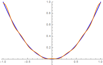
Consider the function \( f (x) = x^2 \) on the interval [-1,1]. Let us take 16 equally spaced points \( x_k = -1 + \frac{2k}{15} , \quad k=0,1,2,\ldots , 15. \) Suppose we want to find the trigonometric polynomial approximation for M = 6 to the 15 data points \( \left\{ (x_k, y_k ) \right\}_{k=1}^{15} . \)

Since the periodic extension is assumed, at a point of discontinuity x = 1, the function value f(1) must be computed using the formula

\[ f(1) = \frac{f(1-0) + f(1+0)}{2} = \frac{1+1}{2} =1. \]
The function \( f (x) = x^2 \) is an even continuous function that is extended periodically; hence the coefficients for the sine terms are all zero (i.e. \( b_j =0 \) for all j). The trigonometric polynomial of degree M = 6 involves only the cosine terms, and we get
\[ a_j = \frac{2}{15} \,\sum_{k=1}^{15} \left( \frac{2k}{15} -1 \right)^2 \cos \left( j\,\pi\, x_k \right) \qquad\mbox{for}\quad j=0,1,2,\ldots , 6 . \]
Now we ask Mathematica for help:
Do[a[j_] := (2/15)* Sum[(2*k/15 - 1)^2 *Cos[j*Pi*(2*k/15 - 1)], {k, 1, 15}], {j, 0, 6}]
Then we calculate the trigonometric polynomial and plot it.
C6[x_] := a[0]/2 + Sum[a[j]*Cos[j*Pi*x], {j, 1, 6}]
Plot[{x^2 , FC6[x]}, {x, -1, 1}, PlotRange -> {-0.1, 1}, PlotStyle -> {{Thick, Blue}, {Thick, Orange}}]
As we see from the graph above, a six term approximation gives a relatively good representation of the given function. ■

Properties of Fourier Coefficients


Let f(x) be an absolutely integrable function on a symmetric interval [−ℓ, ℓ], which we abbreviate as f ∈ 𝔏¹;([−ℓ, ℓ]). Generally speaking, this abbreviation means that function f(x) is integrable in Lebesgue sense. However, you can use Riemann integration instead without any harm. Recall that Fourier coefficients are determined by the Euler--Fourier formulas either in complex form
\[ \hat{f}(n) = \frac{1}{2\ell} \int_{-\ell}^{\ell} f(x)\, e^{-{\bf j} n\pi x/\ell} {\text d} x , \qquad n\in \mathbb{Z} = \left\{ 0, \pm 1, \pm 2, \pm 3, \ldots \right\} ; \tag{3} \]
or in trigonometric form:
\begin{align*} % a_0 &= a_0 (f) = \frac{1}{\ell} \int_{-\ell}^{\ell} f(x)\,{\text d} x , %\notag % \\ a_k &= a_k (f) = \frac{1}{\ell} \int_{-\ell}^{\ell} f(x)\, \cos \left( \frac{k \pi x}{\ell} \right) {\text d} x , \qquad k= 0, 1, 2, 3, \ldots ; \tag{5} \\ b_k &= b_k (f) = \frac{1}{\ell} \int_{-\ell}^{\ell} f(x)\, \sin \left( \frac{k \pi x}{\ell} \right) {\text d} x , \qquad k= 1, 2, 3, \ldots . \notag \end{align*}
We list some basic properties of Fourier coefficients that follow from their definition.
  1. Fourier coefficients are bounded. Specifically
    \[ \left\vert a_k \right\vert , \left\vert b_k \right\vert \le \frac{1}{\ell} \int_{-\ell}^{\ell} \left\vert f(x) \right\vert {\text d} x , \qquad \left\vert \hat{f}(n) \right\vert \le \frac{1}{2\ell} \int_{-\ell}^{\ell} \left\vert f(x) \right\vert {\text d} x . \]
  2. Linearity: If f, g ∈ 𝔏¹([−ℓ, ℓ]), and α, β are arbitrary scalars (real or complex), then
    \[ a_k \left( \alpha f + \beta g \right) = \alpha\,a_k (f) + \beta\,a_k (g) , \qquad b_k \left( \alpha f + \beta g \right) = \alpha\,b_k (f) + \beta\,b_k (g) . \]
  3. If periodic function f(x) has a continuous derivative on [−ℓ, ℓ], then Fourier coefficient of f and its derivative are related according to the following relations:
    \[ a_k (f) = -\frac{1}{k}\,b_k (f') , \qquad b_k (f) = \frac{1}{k}\,a_k (f') , \qquad \hat{f}(\pm n) = \mp \frac{\bf j}{n} \,\hat{f'}(n) . \]
  4. If f has a parity, its Fourier coefficients take special forms:
    • If f(x) is even on symmetric interval [−ℓ, ℓ], then all coefficients bk = 0 and
      \[ a_k = \frac{2}{\ell} \int_0^{\ell} f(x)\,\cos \left( \frac{k\pi x}{\ell} \right) {\text d} x , \qquad k=0,1,2,3,\ldots . \]
    • If f(x) is odd on symmetric interval [−ℓ, ℓ], then all coefficients 𝑎k = 0 and
      \[ b_k = \frac{2}{\ell} \int_0^{\ell} f(x)\,\sin\left( \frac{k\pi x}{\ell} \right) {\text d} x , \qquad k=1,2,3,\ldots . \]
  5. Fourier coefficients do not depend on values of function f(x) at discrete number of points within closed interval [−ℓ, ℓ].

Example 9: We start with the power function p3(x) = x³. Expanding it into Fourier series, we get

\[ x^3 = -\frac{2 \ell^3}{\pi^3} \sum_{n\ge 1} \frac{n^2 \pi^2 -6}{n^3} \left( -1 \right)^n \sin \left( \frac{n \pi x}{\ell} \right) . \]
Integrate[x^3*Sin[n*Pi*x/L], {x, -L, L}]/L
-((2 L^3 (n \[Pi] (-6 + n^2 \[Pi]^2) Cos[n \[Pi]] - 3 (-2 + n^2 \[Pi]^2) Sin[n \[Pi]]))/(n^4 \[Pi]^4))
The Fourier series for x³ converges very slowly.
\[ x^4 = \frac{\ell^4}{5} + \frac{8 \ell^4}{\pi^4} \sum_{n\ge 1} \frac{n^2 \pi^2 -6}{n^4} \left( -1 \right)^n \cos \left( \frac{n \pi x}{\ell} \right) . \]
Integrate[x^4*Cos[n*Pi*x/L], {x, -L, L}]/L
(2 L^4 (4 n \[Pi] (-6 + n^2 \[Pi]^2) Cos[ n \[Pi]] + (24 - 12 n^2 \[Pi]^2 + n^4 \[Pi]^4) Sin[ n \[Pi]]))/(n^5 \[Pi]^5)
So the Fourier series for x4 converges uniformely.

\[ x^5 = -\frac{2 \ell^5}{\pi^5} \sum_{n\ge 1} \frac{n^6 \pi^6 - 42 n^4 \pi^4 + 840 n^2 \pi^2 -5040}{n^7} \left( -1 \right)^n \sin \left( \frac{n \pi x}{\ell} \right) . \]
\[ x^6 = \frac{\ell^6}{7} + \frac{12 \ell^6}{\pi^6} \sum_{n\ge 1} \frac{n^4 \pi^4 -20 n^2 \pi^2 +120}{n^6} \left( -1 \right)^n \cos \left( \frac{n \pi x}{\ell} \right) . \]
\[ x^7 = -\frac{2 \ell^7}{\pi^7} \sum_{n\ge 1} \frac{n^4 \pi^4 -10 n^2 \pi^2 + 120}{n^5} \left( -1 \right)^n \sin \left( \frac{n \pi x}{\ell} \right) . \]
These examples of the Fourier series allow us to make an observation. The Fourier series for monomians with even powers converge uniformly as there general term decreases as 1/n². However, for odd poweers, Fourier series converge but slowly. ■
Riemann--Lebesgue lemma: For every Riemann intagrable function f(x) on interval [−ℓ, ℓ],
\[ \lim_{\nu\to\infty} \int_{-\ell}^{\ell} f(x)\,\cos (\nu x)\,{\text d}x = \lim_{\nu\to\infty} \int_{-\ell}^{\ell} f(x)\,\sin (\nu x)\,{\text d}x = \lim_{\nu\to\infty} \int_{-\ell}^{\ell} f(x)\,e^{{\bf j}\nu x}\,{\text d}x =0. \]
For any real number 𝑎, we define f𝑎(x) = f(x − 𝑎). Its Fourier coefficient is given by
\[ \hat{f}_a (n) = \frac{1}{2\pi} \int_0^{2\pi} f_a (\xi )\,e^{-{\bf j}n\xi} {\text d}\xi = \frac{1}{2\pi} \int_0^{2\pi} f(\xi -a)\,e^{-{\bf j}n\xi} {\text d}\xi , \]
where j is the imaginary unit on complex plane ℂ, so j² = −1. Let t = ξ − 𝑎; the limits of integration do not change as f is assumed to be 2π-periodic function, so we have
\begin{align*} \hat{f}_a (n) &= \frac{1}{2\pi} \int_0^{2\pi} f(t)\,e^{-{\bf j} n \left( t+a \right)} {\text d} t \\ &= \frac{1}{2\pi}\, e^{-{\bf j}na} \int_0^{2\pi} f(t)\,e^{-{\bf j} n t} {\text d}t = e^{-{\bf j}na} \hat{f} (n) . \end{align*}
Now, choose 𝑎 = π/n. Then \( e^{-{\bf j}na} = -1, \) for such 𝑎, and we have
\begin{align*} 2\left\vert \hat{f} (n) \right\vert &= \left\vert \hat{f} (n) - e^{-{\bf j} n a} \hat{f}(n) \right\vert \\ &= \left\vert \hat{f} (n) - \hat{f}_a (n) \right\vert \\ &= \left\vert \frac{1}{2\pi} \int_0^{2\pi} f(t)\,e^{-{\bf j}nt} - \frac{1}{2\pi} \int_0^{2\pi} f(t -a)\,e^{-{\bf j}nt} \right\vert \\ &= \frac{1}{2\pi} \left\vert \int_0^{2\pi} \left[ f(t) - f(t-a) \right] e^{-{\bf j}nt} \right\vert {\text d} t \\ & \le \int_0^{2\pi} \left\vert f(t) - f(t-a) \right\vert {\text d}t . \end{align*}
Note that 𝑎 → 0 as n → ∞.

If f is a continuous function (it is abbreviated as fC0), then \( \left\vert f(t) - f(t-a) \right\vert \to 0 \) for every t ∈ [−ℓ, ℓ]. Hence, by the Dominated Convergent Theorem,

\[ \lim_{n\to\infty} \int_{-\ell}^{\ell} \left\vert f(t) - f\left( t - \frac{\pi}{n} \right) \right\vert {\text d} t = 0 . \]
In general, if f ∈ 𝔏¹, then there exists continuous function g(x) such that for arbitrary positive ε, \( \| f(x) - g(x) \|_1 < \varepsilon \) Take K large enough so that \( \left\vert \hat{g}(k) \right\vert < \varepsilon /2 \) whenever |k| ≥ K. Then
\[ \left\vert \hat{f}(n) \right\vert \le \left\vert \hat{f}(n) - \hat{g} (n) \right\vert + \left\vert \hat{g}(n) \right\vert \le \| f - g \|_1 + \frac{\varepsilon}{2} < \varepsilon , \qquad \mbox{with} \quad \|f \|_1 = \int_{-\ell}^{\ell} \left\vert f(x) \right\vert {\text d}x . \]
The Riemann-Lebesgue lemma is a particular case of the following affirmation.
Lemma 2: Let f(x) be integrable, g(x) be bounded, both periodic. Then
\[ \frac{1}{2\pi} \int_0^{2\pi} f(x)\,g(\nu x)\,{\text d}x \ \mapsto \ \frac{1}{2\pi} \int_0^{2\pi} f(x)\,{\text d}x \,\frac{1}{2\pi} \int_0^{2\pi} g(x)\,{\text d}x \qquad\mbox{as } \quad \nu \to \infty . \]

The following two statements belong to slightly advanced material that is covered in section on mean convergence.

Theorem 4 (Bessel's inequality): Suppose that f(x) is square integrable on the interval [0, T]. Let 𝑎n, bn and \( \hat{f}(n) \) be the Fourier coefficients defined by Eq.\eqref{EqFourier.4} and Eq.\eqref{EqFourier.2}, respectively. Then
\begin{equation} \frac{1}{2} \left\vert a_0 \right\vert^2 + \sum_{n\ge 1} \left( \left\vert a_n \right\vert^2 + \left\vert b_n \right\vert^2 \right) = 2 \sum_{n= -\infty}^{\infty} \left\vert \hat{f}(n) \right\vert^2 \le \frac{2}{T} \int_0^T \left\vert f(x) \right\vert^2 {\text d} x . \end{equation}

This inequality was derived by Friedrich Wilhelm Bessel in 1828.
Although its proof was given in section on orthogonal expansions, we repeat it for pedagogical reasons.

Let SN(f; x) be a partial Fourier sum of function f(x) in exponential form

\[ S_N (f; x) = \sum_{n=-N}^{N} \hat{f}(n)\,e^{{\bf j}\pi nx/\ell} \]
or in trigonometric form
\[ S_N (f; x) = \frac{a_0}{2} + \sum_{k=1}^N \left[ a_k \cos \left( \frac{k\pi x}{\ell} \right) + b_k \sin \left( \frac{k\pi x}{\ell} \right) \right] . \]
We observe that
\[ \int_{-\ell}^{\ell} \left\vert S_N (x) \right\vert^2 {\text d} x = \sum_k \left\vert \phi_k \right\vert^2 , \]
where ϕk(x) is either expopnential mode or trigonometric mode. The identity above follows from orthogonality of eigenfunctions:
\[ \int_{-\ell}^{\ell} e^{{\bf j}\pi nx/\ell} e^{{\bf j}\pi kx/\ell} = 0 \qquad \mbox{for} \quad n\ne k . \]
A similar relatin holds for trignometric functions. Therefore,
\[ \int_{-\ell}^{\ell} \left\vert f(x) - S_N (x) \right\vert^2 {\text d} x = \int_{-\ell}^{\ell} \left\vert f(x) \right\vert^2 {\text d} x + \int_{-\ell}^{\ell} \left\vert S_N (x) \right\vert^2 {\text d} x - 2 \Re \int_{-\ell}^{\ell} \overline{f} (x)\,\phi_k (x)\, {\text d} x . \]
Adding and subtracting \( \sum |c_k |^2 , \) we get
\[ \int_{-\ell}^{\ell} \left\vert f(x) - S_N (x) \right\vert^2 {\text d} x = \int_{-\ell}^{\ell} \left\vert f(x) \right\vert^2 {\text d} x - \sum_{k=0}^N \left\vert c_k \right\vert^2 \| \phi_k \|^2 . \]
Since the left-hand side is positive (at least not negative) we obtain the required indequality when N → ∞,
Actually, Bessel's inequlity can be improved and converted into identity, named after Marc-Antoine Parseval (1755--1836) that expresses the energy of a signal in time-domain in terms of the average energy in its frequency components. In 1799, he stated the following theorem, but did not prove (claiming it to be self-evident). It is also known as Rayleigh's energy theorem, or Rayleigh's identity, after John William Strutt, Lord Rayleigh. [Rayleigh, J.W.S. (1889) "On the character of the complete radiation at a given temperature," "Philosophical Magazine", vol. 27, pages 460-469.] Although the term "Parseval's theorem" is often used in applications, the most general form of this property is more properly called the Plancherel theorem. [Plancherel, Michel (1910) "Contribution a l'etude de la representation d'une fonction arbitraire par les integrales définies," "Rendiconti del Circolo Matematico di Palermo", vol. 30, pages 298-335.]
  • Parseval des Chênes, Marc-Antoine "Mémoire sur les séries et sur l'intégration complète d'une équation aux differences partielle linéaire du second ordre, à coefficiens constans" presented before the Académie des Sciences (Paris) on 5 April 1799. This article was published in "Mémoires présentés à l’Institut des Sciences, Lettres et Arts, par divers savans, et lus dans ses assemblées. Sciences, mathématiques et physiques. (Savans étrangers.)", vol. 1, pages 638-648 (1806).
Parseval Theorem: Let f : [𝑎, b] → ℝ (or ℂ) belongs to the Hilbert space 𝔏²[𝑎, b]. Then Parseval's identity holds
\[ \frac{1}{2} \left\vert a_0 \right\vert^2 + \sum_{n\ge 1} \left( \left\vert a_n \right\vert^2 + \left\vert b_n \right\vert^2 \right) = 2 \sum_{n= -\infty}^{\infty} \left\vert \hat{f}(n) \right\vert^2 = \frac{2}{T} \int_0^T \left\vert f(x) \right\vert^2 {\text d} x . \]
where the Fourier coefficients 𝑎n, bn and \( \hat{f}(n) \) are defined by Eq.\eqref{EqFourier.4} and Eq.\eqref{EqFourier.2}, respectively.
Parseval's identity is a fundamental result on the summability of the Fourier series of a function. It actually establishes completeness of the set of eigenfunctions of the Sturm--Liouville operator L2. Parseval's identity is closely related to the Riesz–Fischer theorem.

Example 10: We consider the power function \( f(x) \left( x^2 - \ell^2 \right)^2 . \) Expanding it into Fourier series, we get

\[ \left( x^2 - \ell^2 \right)^2 = \frac{2\ell^2}{3} + \frac{4 \ell^2}{\pi^2} \sun_{n\ge 1} \frac{(-1)^n}{n^2} \,\cos \left( \frac{n\pi x}{\ell} \right) . \]
To verify Parseval's identity for this function, we first calculate its square norm:
\[ \frac{1}{\ell} \,\| f \|^2 = \frac{1}{\ell} \int_{-L}^L \left( x^2 - \ell^2 \right)^2 {\text d}x = \frac{16}{15}\,\ell^4 . \]
Integrate[(x^2 - L^2)^2, {x, -L, L}]/L
(16 L^4)/15
This number must be equal to the sum of squares of Fourier coefficients:
\[ \frac{16}{15}\,\ell^4 = \frac{8\,\ell^4}{9} + \frac{16 \ell^4}{\pi^4} \sum_{n\ge 1} \frac{1}{n^4} . \]
This equation is simplified to
\[ \sum_{n\ge 1} \frac{1}{n^4} = . \]


Example 10B: Here is another qadratic function (on interval −ℓ < x < ℓ):

\[ x \left( \ell -x \right) = \frac{\ell^2}{3} - \frac{4\ell^2}{\pi^2} \sum_{n\ge 1} \frac{(-1)^n}{n^2} \,\cos \left( \frac{n\pi x}{\ell} \right) - \frac{2\ell^2}{\pi} \sum_{n\ge 1} \frac{(-1)^n}{n^2} \,\sin \left( \frac{n\pi x}{\ell} \right) . \]
Integrate[x*(L - x)*Cos[n*Pi*x/L], {x, -L, L}]/L
-((2 L^2 (2 n \[Pi] Cos[n \[Pi]] + (-2 + n^2 \[Pi]^2) Sin[n \[Pi]]))/( n^3 \[Pi]^3))
Integrate[x*(L - x)*Sin[n*Pi*x/L], {x, -L, L}]/L
-((2 L^2 (n \[Pi] Cos[n \[Pi]] - Sin[n \[Pi]]))/(n^2 \[Pi]^2))
The norm of this function is
\[ \| f \|^2 = \int_{-\ell}^{\ell} x^2 \left( \ell -x \right)^2 {\text d} x = \frac{16}{15}, \ell^5 . \]
Application of Parseval's identity yields
\[ \frac{16}{15}, \ell^4 = \frac{2\ell^4}{9} + \frac{16 \ell^4}{\pi^4} \sum_{n\ge 1} \frac{1}{n^4} + \frac{4\ell^4}{\pi^2} \sum_{n\ge 1} \frac{1}{n^2} . \]
Some simplification yields
\[ \frac{16}{\pi^4} \sum_{n\ge 1} \frac{1}{n^4} + \frac{4}{\pi^2} \sum_{n\ge 1} \frac{1}{n^2} = \]
End of Example 11


Order of Decay of Fourier Coefficients


We investigate the interplay between the smoothness of a function and the decay of its Fourier coefficients. Let us consider a function f(x) having N continuous derivatives on [−ℓ, ℓ]. The integrals in Euler--Fourier formulas \eqref{EqFourier.2} and \eqref{EqFourier.4} can be integrated by parts N times. Taking one coefficient, say 𝑎k, and integrate by parts twice, we obtain
\begin{align*} a_k &= \frac{1}{\ell} \int_{-\ell}^{\ell} f(x)\,\cos \left( \frac{k\pi x}{\ell}\right) {\text d} x = \frac{1}{k\pi} \int_{-\ell}^{\ell} f(x)\,{\text d}\left( \sin\frac{k\pi x}{\ell} \right) \\ &= \frac{1}{k\pi} \left[ f(x)\,\sin\frac{k\pi x}{\ell} \right]_{x=-\ell}^{x=\ell} - \frac{1}{k\pi} \int_{-\ell}^{\ell} f'(x)\,\sin \left( \frac{k\pi x}{\ell}\right) {\text d} x \\ &= \frac{\ell}{(k\pi )^2} \left[ f'(x)\,\cos\frac{k\pi x}{\ell} \right]_{x=-\ell}^{x=\ell} + \frac{\ell}{(k\pi )^2} \int_{-\ell}^{\ell} f''(x)\,\cos \left( \frac{k\pi x}{\ell}\right) {\text d} x . \end{align*}
So we see that if function f(x) has one periodic derivative and the second derivative is integrable, the Fourier coefficients decay as 1/k². Clearly, this process can be continued until the N-th differential appears in the integral, but useful information can be greened from these expressions.

Theorem 6: If a periodic function f(x) is continuous and has continuous periodic derivatives up to the (N−1)-st order and if its N-th derivative is integrable on interval [−ℓ, ℓ], then its Fourier coefficients can be estimated by
\[ 2 \left\vert \hat{f}(n) \right\vert = \sqrt{a_n^2 + b_n^2} \le \frac{K}{n^N} , \]
where K is a positive constant.

Example 11: ?????????????


Discretization


Euler--Fourier formulas \eqref{EqFourier.2} or \eqref{EqFourier.4} provide discretization of a corresponding function f, so they can be considered as transferring a signal into discrete sets:

\[ \vert\,f \,\rangle = \left[ \cdots , \hat{f}(-n) , \cdots , \hat{f}(-1) , \ \hat{f}(0) ,\ \hat{f}(1) ,\cdots , \hat{f}(n) , \cdots \right] \]
or
\[ \vert\,f \,\rangle = \left( \begin{bmatrix} a_0 \\ 0 \end{bmatrix} , \ \begin{bmatrix} a_1 \\ b_1 \end{bmatrix} \ \begin{bmatrix} a_2 \\ b_2 \end{bmatrix} , \ \begin{bmatrix} a_3 \\ b_3 \end{bmatrix} , \ \cdots \right) = \left[ \cdots , b_k, b_{k-1} , \cdots , b_1 , a_0, a_1 , a_2 , \cdots , a_k , \cdots \right] . \]
Fourier series formulas
\[ f(x) \,\sim\, \mbox{P.V.}\sum_{n=-\infty}^{+\infty} \hat{f}(n)\, e^{n{\bf j} \pi x/\ell} = \lim_{N\to \infty} \sum_{n=-N}^{N} \hat{f}(n)\, e^{n{\bf j} \pi x/\ell} = S[f], \tag{2} \]
or
\[ f(x) \,\sim\, \frac{a_0}{2} + \sum_{k=1}^{\infty} \left[ a_k \cos \left( \frac{k \pi x}{\ell} \right) + b_k \sin \left( \frac{k \pi x}{\ell} \right) \right] = S[f], \tag{4} \]
provide the inverse transformation from discrete (or digital) form ∣f ⟩ into analog form. Restoration of a function f(x) from its discrete set ∣f ⟩ is an ill-posed problem. It depends not only on properties of the function f(x), but also on the definition of convergence of infinite series.

Example 12: Let us consider a piecewise continuous function

\[ f(x) = \begin{cases} 0, & \ \mbox{ for} \quad -2 < x < 0 , \\ -1/2 , & \ \mbox{ for} \quad x=0, \\ (x-1)^2 , & \ \mbox{ for} \quad 0 < x < 2 . \end{cases} \tag{14.1} \]
End of Example 11

Convergence of Fourier Series


Is it true that partial Fourier sums SN(f; x) converge to the function f(x) as N → ∞? In general, that is far too much to hope for because restoration of a function from its Fourier coefficients ∣f ⟩ is an ill-posed problem. Not every function is suitable for a Fourier series expansion, but those that satisfy some conditions. For example, the tangent function tan(x) cannot be expanded into the Fourier series on any interval containing the roots of the equation cos(x) = 0 simply because the Fourier coefficients do not exist. For certain kinds of functions convergence is assured; but we will see that some functions are so weird that SN(f; x) diverges for every x.

It was a surprise when the German mathematician Paul David Gustav du Bois-Reymond (1831--1889) was able in 1873 to construct a continuous function whose Fourier series diverges at a point. Despite this negative result, we might ask what happens if we add more smoothness conditions on a generating function. Although we don't know necessary and sufficient conditions for a function to be expanded into a Fourier series, we know some sufficient conditions that guarantee a Fourier series expansion. The Fourier series does not exist unless, for example, 𝑎0 exists (i.e., \( \left\vert \int_{-\ell}^{\ell} f(x) \,{\text d}x \right\vert < \infty \) ). Even when the integral for 𝑎0 exists, the Fourier series may converge to another function.

Example 13:

End of Example 11

All expansion formulas involve infinite series; their convergence is based on properties of partial sums, either \eqref{EqFourier.1}

\[ S_N (f;x) = \sum_{k=-N}^{N} \hat{f}(k)\, e^{k{\bf j} \pi x/\ell} \tag{6} \]
for complex-valued functions, or \eqref{EqFourier.3}
\[ S_N (f;x) = \frac{a_0}{2} + \sum_{k=1}^{N} \left[ a_k \cos \frac{k \pi x}{\ell} + b_k \sin \frac{k \pi x}{\ell} \right] , \tag{7} \]
for real-valued functions. A Fourier series converges when its partial sums SN(f; x) approach a limit in some sense; it exists not for arbitrary functions. Since a Fourier series is a series involving trigonometric functions, the corresponding partial sums depend on a parameter x∈ℝ. Upon considering partial sums for every value of x, we arrive at the pointwise convergence of the series of functions (in our case, trigonometric functions). A pointwise convergence of Fourier series is a very delicate matter, which we touch in convergence section.

A natural question that comes to your mind is whether the series \eqref{EqFourier.1} or \eqref{EqFourier.3} converges and if they converge, do they converge to generating function f(x)? Mathematicians tell us that none of these questions have simple answers. We still do not know the exact conditions to fully identify the class of functions whose Fourier series pointwise converge to the same functions. Identification of the function from its Fourier coefficients is an ill-posed problem, and in many cases it requires a regularization. One of such possible regularization is discussed in Cesàro summation section. Nonetheless, Fourier series usually work quite well (especially in situations where they arise from physical problems).

We leave discussion of convergence of Fourier series to two following sections; however, here we use a simple sufficient conditions that is easy to verity.

Theorem 7: Every function from the domain of a self-adjoint differential operator of second order can be expanded into uniformly convergent Fourier series over the set of its eigenfunctions.
The proof of this theorem is based on reduction of the problem to an integral equation. Then using the Hilbert--Schmidt theorem, a function is expanded into series over eigenfunctions. See details in a course on integral equations.

Recall that the domain of a linear differential operator of order n consists of all functions that have continuous derivatives up to the order n and satisfy the differential equation and the boundary conditions that generate the linear operator. Since a Fourier series is an expansion over eigenfunctions of the second order differential operator \( L_2 \left[ \texttt{D} \right] = - \texttt{D}^2 = - {\text d}^2 /{\text d}x^2 , \) subject to the periodic boundary conditions, the domain of L2 consists of all periodic twice differentiable functions. The equation \( L_2 \left[ \texttt{D} \right] y = \lambda\, y \) to be satisfied requires that the second derivative is also a periodic function.

Theorem 8: If a periodic function f possesses two continuous derivatives, then its Fourier series S[f](x) converges uniformely to f(x).

Remember that a Fourier series is also generated by the first order self-adjoint differential operator \( \hat{p} = - {\bf j}\,\texttt{D} , \) with j being the imaginary unit on ℂ. However, the Sturm--Liouville theory is applicable only to the second order self-adjoint differential operators, and its application to the first order operators requires further development. Nevertheless, we will see later that existence of periodic continuous derivative will be sufficient for convergence of the Fourier series.

Example 14: We consider the the function f(x) = (cosx)4 on interval [−π, π]. Expanding it into Fourier series, we get

\[ \cos^4 x = \frac{3}{2} + \frac{1}{2}\,\cos 2x + \frac{1}{8}\,\cos 4x . \]
Integrate[(Cos[x])^4, {x, -Pi, Pi}]/Pi
3/4
Integrate[(Cos[x])^4*Cos[n*x], {x, -Pi, Pi}]/Pi
(2 (24 - 16 n^2 + n^4) Sin[n \[Pi]])/(n (64 - 20 n^2 + n^4) \[Pi])
We check the answer with Mathematica:
S11[x_] = 3/2 + Cos[2*x]/2 + Cos[4*x]/8;
p111 = Plot[{S11[t]}, {t, -\[Pi], \[Pi]}, PlotStyle -> {Thickness[0.02], Purple}];
p112 = Plot[(Cos[t])^4, {t, -\[Pi], \[Pi]}, PlotStyle -> {Thickness[0.007], Blue}];
Show[p111, p112]

Uniqueness of Fourier Series


Since the Fourier coefficients of function f(x) are determined through integrals \eqref{EqFourier.2} or \eqref{EqFourier.4}, it requires f(x) to be integrable, so f ∈ 𝔏¹. Assuming that the Fourier series for f(x) converges to f in an appropriate sense, the natural question should appear: is this series unique? This would lead to the following statement: if \( \hat{f}(n) = 0 \) for all n ∈ ℤ, then f(x) ≡ 0. This assertion cannot be correct without reservation because calculating Fourier coefficients requires integration, and we know that any two functions that differ at finitely many (or discrete) points have the same Fourier series. However, we do have the following positive result.

Theorem 9: Let f be a periodic integrable on finite interval [−ℓ, ℓ] function. Suppose that f is 0 in a neighbourhood of x; that is, there exists δ >0 such that f(t) ≡ 0 for all t∈(x−δ, x+δ). Then the partial Fourier sum SN(f; x) → 0 as N → ∞.
This result is significant in that while the Fourier coefficients \( \hat{f}(n) \) depends on the values of f globally— that is, to calculate \( \hat{f}(n) \) one needs to know f everywhere withing the full interval — the convergence of SN(f; x) only depends on a local neighbourhood of that point.
We compute
\begin{align*} S_N (f; x) &= \frac{1}{2\pi} \int_{-\pi}^{\pi} f(y)\,D_N (x-y)\,{\text d}y \\ &= \frac{1}{2\pi} \int_{-\pi}^{\pi} f(x-y)\,D_N (y)\,{\text d}y \\ &= \frac{1}{2\pi} \int_{[-\pi , \pi] \setminus [-\delta , \delta ]} f(x-y)\,D_N (y)\,{\text d}y + \frac{1}{2\pi} \int_{ [-\delta , \delta ]} f(x-y)\,D_N (y)\,{\text d}y \\ &= \frac{1}{2\pi} \int_{[-\pi , \pi] \setminus [-\delta , \delta ]} f(x-y)\, \frac{\sin \left( N + \tfrac{1}{2} \right) y}{\sin\tfrac{y}{2}} . \end{align*}
Now mapping
\[ y \mapsto \frac{f(x-y)}{\sin\tfrac{y}{2}} \]
is an 𝔏¹ function on \( [-\pi , \pi] \setminus [-\delta , \delta ] , \) so
\begin{align*} S_N (f; x) &= \frac{1}{2\pi} \int_{-\pi}^{\pi} \chi_S (y)\, \frac{f(x-y)}{\sin \tfrac{y}{2}} \cdot \frac{e^{{\bf j} \left( N + \tfrac{1}{2} \right) y} - e^{-{\bf j} \left( N + \tfrac{1}{2} \right) y} }{2{\bf j}}\, {\text d}y \\ &= \frac{1}{2\pi} \cdot \frac{1}{2{\bf j}} \int_{-\pi}^{\pi} \chi_S (y)\, \frac{f(x-y)}{\sin \tfrac{y}{2}} \cdot e^{{\bf j} \left( N + \tfrac{1}{2} \right) y} {\text d}y - \frac{1}{2\pi} \cdot \frac{1}{2{\bf j}} \int_{-\pi}^{\pi} \chi_S (y)\, \frac{f(x-y)}{\sin \tfrac{y}{2}} \cdot e^{-{\bf j} \left( N + \tfrac{1}{2} \right) y} {\text d}y \end{align*}
Setting
\[ g(y) = \chi_S (y) \, \frac{f(x-y)}{\sin \tfrac{y}{2}} \cdot e^{{\bf j} y/2} \qquad\mbox{and} \qquad h(y) = \chi_S (y) \, \frac{f(x-y)}{\sin \tfrac{y}{2}} \cdot e^{-{\bf j} y/2} \]
we see that the two terms are nothing but Fourier coefficients of g and h, so that
\[ S_N (f; x) = \frac{1}{2\pi}\left[ \hat{g}(-N) - \hat{h}(N) \right] \,\to 0 \qquad\mbox{as} \quad N \to \infty \]
by the Riemann-Lebesgue lemma.
Uniqueness Theorem: Suppose that f(x) is a periodic integrable function on the interval [−ℓ, ℓ] (it is abbreviated as f∈𝔏¹) with Fourier coefficients \( \hat{f}(n) =0 \) for all n ∈ ℤ={ 0, ±1, ±2, … }. Then f(ξ) = 0 whenever f(x) is continuous at the point ξ ∈[−ℓ, ℓ].
We suppose first that f is real-valued, and argue by contradiction. Assume, without loss of generality, that f is defined on {−π, π] and ξ = 0, with f(ξ) > 0. The idea now is to construct a family of trigonometric polynomials {pk} that “peak” at 0, and so that \( \int p_k (t)\,f(t)\,{\text d}t \to \infty \) as k → ∞. This will be our desired contradiction since these integrals are equal to zero by assumption.

Since f is continuous at 0, we can choose 0 < δ π/2, so that f(ξ) f(0)/2, whenever |ξ| < δ. Let

\[ p(t) = \epsilon + \cos t, \]
where ϵ > 0 is chosen so small that |p(t)| < 1 −ϵ/2, whenever δ ≤ |t| ≤ π. hen, choose a positive η with η < δ so that p ≥ 1 + ϵ/2, for |t| < η. Finally, let
\[ p_k (t) = \left[ p(t) \right]^k , \]
and select B so that |f(t)| < B for all t. This is possible since f is integrable, hence bounded.

By construction, each pk is a trigonometric polynomial, and since \( \hat{f}(n) = 0 \) for all n ∈ ℤ, we must have

\[ \int_{-\pi}^{\pi} f(t)\,p_k (t) \,{\text d}t = 0 \qquad \mbox{for al} \quad k. \]
However, we have the estimate
\[ \left\vert \int_{-\pi}^{\pi} f(t)\,p_k (t) \,{\text d}t \right\vert \le 2\pi B \left( 1 - \epsilon /2 \right)^k . \]
Also, our choice of δ guarantees that p(t) and f(t) are non-negative whenever |t| < δ; thus,
\[ \int_{\eta \le |t| < \delta} f(t)\,p_k (t) \,{\text d}t \ge 0. \]
Finally,
\[ \int_{|t| <\eta} f(t)\,p_k (t) \,{\text d}t \ge 2\eta\,\frac{f(0)}{2} \left( 1 + \epsilon /2 \right)^k . \]
Therefore, \( \int p_k (t) \,f(t)\,{\text d}t \to\infty \) as k → ∞. This concludes the proof when f is real-valued. In general, write f(t) = u(t) + jv(t), where u and v are real-valued. If we define complex conjugate \( \overline{f} (t) = \overline{f(t)}, \) then
\[ u(t) = \frac{f(t) + \overline{f}(t)}{2} \qquad \mbox{and} \qquad v(t) = \frac{f(t) - \overline{f}(t)}{2} , \]
and since \( \hat{\overline{f}}(n) = \overline{\hat{f}(-n)} , \) we conclude that the Fourier coefficients of u and v all vanish; hence f= 0 at its points of continuity.
Corollary 1: If f(x) is a periodic continuous function and its Fourier coefficients are all zero, then f(x) ≡ 0.
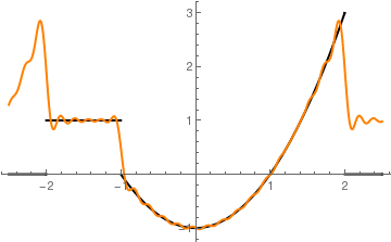
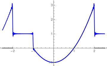
Example 17: Consider the piecewise continuous function on the interval [-2,2]:

\[ f(x) = \begin{cases} 1, & \ \mbox {if } -2 < x < -1 , \\ x^2 -1, & \ \mbox {if } -1< x< 2 , \end{cases} \]
Its Fourier coefficients are evaluated with the aid of Mathematica:
f[x_] = Piecewise[{{1, -2 < x < -1}, {x^2 - 1, -1 < x < 2}}, 0]
Integrate[f[x], {x, -2, 2}]/2
1/2
Other coefficients we find by direct integration:
Simplify[Integrate[f[x]*Sin[n*Pi*x/2], {x, -2, 2}]/2 , Assumptions -> Element[n, Integers]]
-((2 (-1)^n (-4 + n^2 \[Pi]^2) + (8 + n^2 \[Pi]^2) Cos[(n \[Pi])/2] + 4 n \[Pi] Sin[(n \[Pi])/2])/(n^3 \[Pi]^3))
Simplify[Integrate[f[x]*Cos[n*Pi*x/2], {x, -2, 2}]/2 , Assumptions -> Element[n, Integers]]
(8 (-1)^n n \[Pi] + 4 n \[Pi] Cos[(n \[Pi])/2] - (8 + n^2 \[Pi]^2) Sin[(n \[Pi])/ 2])/(n^3 \[Pi]^3)
So
\begin{align*} a_0 &= \frac{1}{2} , \\ a_n &= \frac{8(-1)^n n\pi + 4n\pi \cos \left( \frac{n\pi}{2} \right) - \left( 8 + n^2 \pi^2 \right) \sin \left( \frac{n\pi}{2} \right)}{n^3 \pi^3} , \\ b_n &= - \frac{2 (-1)^n \left( n^2 \pi^2 -4 \right) + \left( 8 + n^2 \pi^2 \right) \cos \left( \frac{n\pi}{2} \right) + 4n\pi\,\sin \left( \frac{n\pi}{2} \right)}{n^3 \pi^3} . \end{align*}
Finally, we build partial Fourier sums with N = 10, 20, and 100 terms
F10[x_] = 1/4 + Sum[(( 8 (-1)^n n \[Pi] + 4 n \[Pi] Cos[(n \[Pi])/2] - (8 + n^2 \[Pi]^2) Sin[(n \[Pi])/ 2])/(n^3 \[Pi]^3))* Cos[n*Pi*x/2] - (( 2 (-1)^n (-4 + n^2 \[Pi]^2) + (8 + n^2 \[Pi]^2) Cos[(n \[Pi])/ 2] + 4 n \[Pi] Sin[(n \[Pi])/2])/(n^3 \[Pi]^3))* Sin[n*Pi*x/2], {n, 1, 10}]
F20[x_] = 1/4 + Sum[(( 8 (-1)^n n \[Pi] + 4 n \[Pi] Cos[(n \[Pi])/2] - (8 + n^2 \[Pi]^2) Sin[(n \[Pi])/ 2])/(n^3 \[Pi]^3))* Cos[n*Pi*x/2] - (( 2 (-1)^n (-4 + n^2 \[Pi]^2) + (8 + n^2 \[Pi]^2) Cos[(n \[Pi])/ 2] + 4 n \[Pi] Sin[(n \[Pi])/2])/(n^3 \[Pi]^3))* Sin[n*Pi*x/2], {n, 1, 20}]
F100[x_] = 1/4 + Sum[(( 8 (-1)^n n \[Pi] + 4 n \[Pi] Cos[(n \[Pi])/2] - (8 + n^2 \[Pi]^2) Sin[(n \[Pi])/ 2])/(n^3 \[Pi]^3))* Cos[n*Pi*x/2] - (( 2 (-1)^n (-4 + n^2 \[Pi]^2) + (8 + n^2 \[Pi]^2) Cos[(n \[Pi])/ 2] + 4 n \[Pi] Sin[(n \[Pi])/2])/(n^3 \[Pi]^3))* Sin[n*Pi*x/2], {n, 1, 100}]
and plot them:
Plot[{f[x], F10[x]}, {x, -2.5, 2.5}, PlotStyle -> {{Thick, Black}, {Thick, Red}}]
Plot[{f[x], F20[x]}, {x, -2.5, 2.5}, PlotStyle -> {{Thick, Black}, {Thick, Orange}}]
Plot[{f[x], F100[x]}, {x, -2.5, 2.5}, PlotStyle -> {{Thick, Black}, {Thick, Blue}}]
   Fourier approximation with 10 terms    Fourier approximation with 20 terms    Fourier approximation with 100 terms
       
   ■

Example 18: Let us consider a periodic step function with period T:

\[ f(x) = \mbox{sign}\left( \sin \frac{2\pi x}{T} \right) = \begin{cases} \phantom{-}1, & \ \mbox{for }\ 0 < x < T /2, \\ -1, & \ \mbox{for }\ T/2 < x < T . \end{cases} \]
Plot[Sign[Sin[Pi*x]], {x, 0, 4}, PlotStyle -> Thick]
Periodic step function with period 2.
Its Fourier series becomes
\[ \mbox{sign}\left( \sin \frac{2\pi x}{T} \right) = \frac{4}{\pi} \sum_{n\ge 1} \frac{1}{2n-1}\,\sin \frac{2\pi x \left( 2n -1 \right)}{T} . \]
      Using Mathematica We plot animation of the Fourier series approximation depending on the number m of terms.
s[x_, m_] = 4*Sum[Sin[Pi*x*(2*n - 1)]/(2*n - 1), {n, 1, m}]/Pi;
animation = Table[Plot[s[x, m], {x, -0.1, 2*Pi + 0.1}, PlotRange -> {-1, 1, 1.1}, PlotStyle -> Thickness[0.008], PlotLabel -> "Fourier approximation depends on " <> ToString[m] <> " terms"], {m, 0, 100, 2}];;
Export["Animation.gif", animation, "AnimationRepetitions" -> 100]
       Fourier series approximation depending on the number of terms. .            Mathematica code


Let χ(x) be the chracteristic function of the interval (−h, h):
\[ \chi (x) = \begin{cases} 1, & \ \mbox{if}\quad -h < x < h, \\ 0, & \ \mbox{otherwise}. \end{cases} \]
Its Fourier series is
\[ S{\chi ](x) = \frac{1}{2}\, a_0 + \sum_{k \ge 1} a_k \cos (kx) , \]
where
\[ a_k = \]
The conjugate function is
\[ \chi^{\ast} (x) = \sum_{k \ge 1} a_k \sin (kx) = \frac{1}{\pi}\,\ln \left\vert \frac{\sin \frac{1}{2} \left( x+h \right)}{\sin \frac{1}{2} \left( x-h \right)} \right\vert . \]
   ■

Operations on Fourier Series


Theorem 11: Let f(x) be an absolutely integrable function on interval [−ℓ, ℓ] and let S[f] be its exponential Fourier series, that is,
\[ f(x) \sim S[f] = \mbox{P.V.} \sum_{n=-\infty}^{+\infty} \hat{f}(n) \, e^{{\bf j}\pi nx/\ell} . \]
Then
  • \[ \overline{f(x)} \sim \mbox{P.V.} \sum_{n=-\infty}^{+\infty} \overline{\hat{f}(n)} \, e^{-{\bf j}\pi nx/\ell} = \sum_{n=-\infty}^{+\infty} \overline{\hat{f}(-n)} \, e^{{\bf j}\pi nx/\ell} ; \]
  • \[ e^{{\bf j}\pi mx/\ell} f(x) \sim \mbox{P.V.} \sum_{n=-\infty}^{+\infty} \overline{\hat{f}(n)} \, e^{-{\bf j}\pi \left( n + m \right) x/\ell} = \sum_{n=-\infty}^{+\infty} \hat{f}(n-m)\, e^{{\bf j}\pi nx/\ell} \]
  • \[ f(x+y) \sim \mbox{P.V.} \sum_{n=-\infty}^{+\infty} \hat{f}(n)\, e^{{\bf j}\pi nx/\ell} \, e^{{\bf j}\pi ny/\ell} . \]
The proofs are simple and straightforward (so we omit them).

Theorem 12: If \( f(x) \sim \sum_{n=-\infty}^{+\infty} \alpha_n e^{{\bf j}\pi nx/\ell} \) and \( g(x) \sim \sum_{n=-\infty}^{+\infty} \beta_n e^{{\bf j}\pi nx/\ell} , \) then
\[ \sum_{n=-\infty}^{+\infty} \alpha_n \beta_n e^{{\bf j}\pi nx/\ell} = \frac{1}{2\ell}\,f\star g (x) = \frac{1}{2\ell} \int_{-\ell}^{\ell} f(x-y)\,g(y) \,{\text d} y . \]
We show first that the convolution integral exists for almost all x. We can assume that functions f and g are real-valued functions. Without any loss of generality, we can assume that both functions are not negative. Then
\[ \int_{-\ell}^{\ell} {\text d}x \int_{-\ell}^{\ell} {\text d} y\, f(x-y)\,g(y) = \int_{-\ell}^{\ell} {\text d}y\, g(y) \, \int_{-\ell}^{\ell} {\text d} x\, f(x-y) = \int_{-\ell}^{\ell} {\text d}y\, g(y) \, \int_{-\ell}^{\ell} {\text d} x\, f(x) . \]
The operations performed here are justified because the kernel of convolution, f( x - y) g(y) is measurable in the (x, y) as a product of two measarable functions. Allso, the order of integration is irrelevant.

The kernel f(xy) g(y) is integrable over the square 0 ≤ x, y ≤ 2ℓ. Thus, for arbitrary integrable functions, \( \left\vert f(x-y)\,g(y)\,e^{{\bf j} n\pi x/\ell} \right\vert \) is integrable over the square and the following argument is also legimate:

\begin{align*} \frac{1}{2\ell} \int_{-\ell}^{\ell} \left( f \star g \right) e^{-{\bf j}\pi nx/\ell} {\text d} x &= \frac{1}{2\ell} \int_{-\ell}^{\ell} \left\{ \frac{1}{2\ell} \int_{-\ell}^{\ell} f(x-y)\, e^{-{\bf j}\pi n\left( x-y \right) /\ell} g(y)\, e^{-{\bf j}\pi ny/\ell} {\text d} y \right\} {\text d} x \\ &= \frac{1}{2\ell} \int_{-\ell}^{\ell} g(y)\,e^{-{\bf j}\pi ny/\ell} {\text d} y \left\{ \frac{1}{2\ell} \int_{-\ell}^{\ell} f(x-y)\, e^{-{\bf j}\pi n\left( x-y \right) /\ell} {\text d} x \right\} = \alpha_n \beta_n . \end{align*}


Term-by-term differentiation of infinite series


Not every Fourier series can be term-by-term differentiated, but those that correspond to functions having derivatives expanded into Fourier series. Term-by-term differentiation is not justified for functions having an unbounded jump discontinuity. In mathematics, there is a special class of functions, called absolute continuous that have derivatives almost everywhere.

Suppose that a periodic function f(x) is an integral, i.e., f(x) is absolutely continuous. Integrating by parts gives

\[ \hat{f}(n) = \frac{1}{2\ell} \int_{-\ell}^{\ell} f(x)\, e^{-{\bf j} \pi nx/\ell} {\text d} x = \frac{1}{2n\pi} \int_{-\ell}^{\ell} f' (x)\, e^{-{\bf j} \pi nx/\ell} {\text d} x = \frac{1}{{\bf j}n} \,\hat{f'}(n) , \qquad n\ne 0, \]
so that \( \hat{f'}(n) = {\bf j}n\,\hat{f}(n) , \) where \( \hat{f'}(n) \) is the Fourier coefficient of the derivative of f(x). Since f(x) is periodic, \( \hat{f'}(0) = 0. \) Similar for trigonometric series \eqref{EqFourier.3}, we have
\begin{align*} a_k (f') &= \frac{1}{\ell} \int_{-\ell}^{\ell} f' (x)\,\cos \left( \frac{k\pi x}{\ell} \right) {\text d} x = \left. \frac{1}{\ell} f (x)\,\cos \left( \frac{k\pi x}{\ell} \right)\right\vert_{x=-\ell}^{x=\ell} + \frac{n\pi}{\ell^2} \int_{-\ell}^{\ell} f(x) \,\sin \left( \frac{k\pi x}{\ell} \right) {\text d} x \\ &= \frac{n\pi}{\ell^2} \int_{-\ell}^{\ell} f(x) \,\sin \left( \frac{k\pi x}{\ell} \right) {\text d} x , \\ b_k (f') &= \frac{1}{\ell} \int_{-\ell}^{\ell} f' (x)\,\sin \left( \frac{k\pi x}{\ell} \right) {\text d} x = \left. \frac{1}{\ell} f (x)\,\sin \left( \frac{k\pi x}{\ell} \right)\right\vert_{x=-\ell}^{x=\ell} - \frac{n\pi}{\ell^2} \int_{-\ell}^{\ell} f(x) \,\cos \left( \frac{k\pi x}{\ell} \right) {\text d} x \\ &= \frac{n\pi}{\ell^2} \int_{-\ell}^{\ell} f(x) \,\cos \left( \frac{k\pi x}{\ell} \right) {\text d} x , \end{align*}
because f(−ℓ) = f(ℓ). Thus, if S'[f] denotes the result of differentiating S[f] term by term, we have
\[ f' (x) \sim {\mbox P.V.} \,{\bf j} \sum_{n=-\infty}^{+\infty} n\, \hat{f}(n) \, e^{{\bf j}n\pi x/\ell} = \sum_{k\ge 1} n \left( b_k \cos \frac{k\pi x}{\ell} - a_k \sin \frac{k\pi x}{\ell} \right) . \]
This is precisely what would be obtained by differentiating the Fourier series of f(x) term by term. Hence, even though the Fourier series S[f'] of f'(x) may not converge uniformly or even converge at all, it can still be obtained by differentiating the Fourier series S[f] of f(x) term by term.

Theorem 13: If f(x) is m-th integral (m = 1, 2, …), then \( S^{(m)}[f] = S[f^{(m)}] , \) where S[f] is the Fourier series for function f.
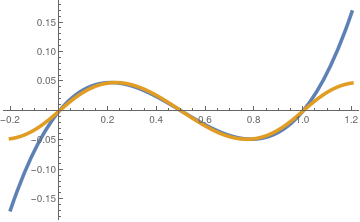
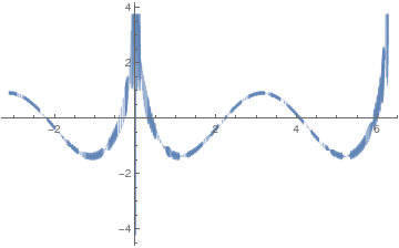
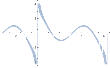
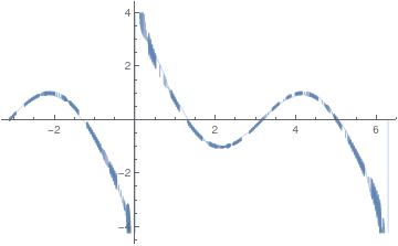
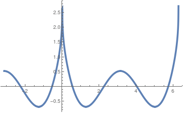
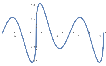
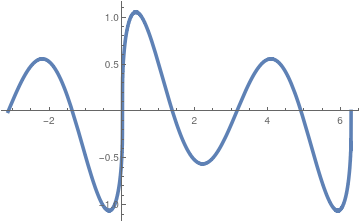
Example 19: Let us consider a function f(x) = x on the interval [0, ℓ]. Its Fourier series is

\[ x = \sum_{n\ge 1} \frac{2\ell}{n\pi} \,(-1)^{n+1} \,\sin \left( \frac{n\pi x}{\ell} \right) , \qquad \ell < x < \ell . \]
You will learn later in the even and odd section how to construct this series and determine the coefficients, but now you have to trust me or plot partial sums to verify the identity. If we differentiate the function on the left-hand side, then we get the function 1. However, if we formally differentiate term by term the function on the right, then we arrive at
\[ 1 \stackrel{?}{=} 2 \sum_{n\ge 1} (-1)^{n+1} \,\cos \left( \frac{n\pi x}{\ell} \right) , \qquad \ell < x < \ell . \]
The series at the left does not converge because its general term does not tern to zero. However, we will see later that if we use another definition of convergence, called Cesàro summation, the right-hand side series converges to 1. If we formally apply geometric series formula (see Example 2 in Cesàro summation section)
\[ \sum_{n\ge 1} q^n = \frac{q}{1-q} , \qquad \mbox{with} \quad q = -e^{{\bf j}x} , \]
we obtain
\begin{align*} \sum_{n\ge 1} (-1)^{n+1} \,\cos \left( nx \right) &= - \Re \sum_{n\ge 1} (-1)^{n} \, e^{{\bf j}nx} = - \Re \sum_{n\ge 1} \left( -e^{{\bf j}x} \right)^n - \\ &= - \Re \frac{-e^{{\bf j}x}}{1 + e^{{\bf j}x}} = - \Re \frac{-e^{{\bf j}x} \left( 1 + e^{-{\bf j}x} \right)}{\left( 1 + e^{{\bf j}x} \right) \left( 1 + e^{-{\bf j}x} \right)} = - \Re \frac{- e^{{\bf j}x} -1}{2 + 2\,\cos x} \\ &= \Re \frac{1 + e^{{\bf j}x}}{2 \left( 1 + \cos x \right)} = \frac{1 + \cos x}{2 + 2\,\cos x} = \frac{1}{2} . \end{align*}


However, wait a minute. There exist another Fourier series for the same function (if you open the same section):
\[ x = \frac{\ell}{2} - \frac{4\ell}{\pi^2} \sum_{n\ge 1} \frac{1}{n^2} \,\cos \left( \frac{n\pi x}{\ell} \right) , \qquad \ell < x < \ell . \]
Fourier sine series of the derivative f'(x) = 1 can be obtained by term-by-term differentiation of the Fourier cosine series of f(x) = x. Assuming that term-by-term differentiation is valid as claimed, it follows that
\[ 1 = \frac{4}{\pi} \sum_{n\ge 1} \frac{1}{n}\, \sin \left( \frac{n\pi x}{\ell} \right) , \qquad \ell < x < \ell , \]
which is, in fact, correct.    ■

Example 20: The Bernoulli polynomials Bn(x) are solutions of the Appell differential equation

\[ \frac{{\text d} p_n (x)}{{\text d}x} = n\,p_{n-1} (x) , \]
which is similar to the power function. We list a few first Bernoulli polynomials:
\begin{align*} B_0 &= 1, \\ B_1 (x) &= x - \frac{1}{2} , \\ B_2 (x) &= x^2 -x + \frac{1}{6} , \\ B_3 (x) &= x^3 - \frac{3}{2}\, x^2 + \frac{1}{2}\, x , \\ B_4 (x) &= x^4 - 2x^3 + x^2 - \frac{1}{30} , \\ B_5 (x) &= x^5 - \frac{5}{2}\,x^4 + \frac{5}{3}\,x^3 - \frac{1}{6}\, x . \end{align*}
Mathematica has a build-in command for evaluation of Bernoulli polynomials.
Table[BernoulliB[k, x], {k, 0,5}]
So we expand Bernoulli's polynomials of order 3 and 4 into Fourier series
2*Integrate[BernoulliB[4, x]*Cos[Pi*n*x], {x, 0, 1}]/1
-((360 n \[Pi] + 360 n \[Pi] Cos[ n \[Pi]] + (-720 + 60 n^2 \[Pi]^2 + n^4 \[Pi]^4) Sin[n \[Pi]])/( 15 n^5 \[Pi]^5))
\[ a_n \left( B_4 \right) = 2 \int_0^1 B_4 (x)\,\cos (n\pi x)\,{\text d} x = -\frac{24}{n^4 \pi^4} - \frac{24}{n^4 \pi^4}\, (-1)^n = - \frac{48}{n^4 \pi^4} \times \begin{cases} 1, & \ \mbox{ if} \quad n = 2k , \\ 0, & \ \mbox{ if} \quad n = 2k +1. \end{cases} \]
Therefore,
\[ B_4 (x) = x^4 - 2x^3 + x^2 - \frac{1}{30} = - \frac{3}{\pi^4} \sum_{k\ge 1} \frac{1}{k^4}\,\cos \left( 2k\pi x \right) . \]
      We plot with Mathematica:
s20[x_] = -3/(1*Pi^4)*Sum[Cos[2*k*Pi*x]/k^4, {k, 1, 20}]; Plot[{BernoulliB[4, x], s20[x]}, {x, -0.2, 1.2}, PlotStyle -> Thickness[0.01]]
        20 term Fourier approximation to Bernoulli's polynomial B4(x).            Mathematica code

Now we expand Bernoulli's polynomial of order 3 into Fourier series
2*Integrate[BernoulliB[3, x]*Sin[Pi*n*x], {x, 0, 1}]/1
(6 n \[Pi] + 6 n \[Pi] Cos[n \[Pi]] + (-12 + n^2 \[Pi]^2) Sin[ n \[Pi]])/(n^4 \[Pi]^4)
\[ b_n \left( B_3 \right) = 2 \int_0^1 B_3 (x)\,\sin (n\pi x)\,{\text d} x = \frac{6}{n^3 \pi^3} + \frac{6}{n^3 \pi^3}\, (-1)^n = \frac{12}{n^3 \pi^3} \times \begin{cases} 1, & \ \mbox{ if} \quad n = 2k , \\ 0, & \ \mbox{ if} \quad n = 2k +1. \end{cases} \]
This yields
\[ B_3 (x) = x^3 - \frac{3}{2}\, x^2 + \frac{1}{2}\, x = \frac{3}{2\pi^3} \sum_{k\ge 1} \frac{1}{k^3}\,\sin \left( 2k\pi x \right) . \]
      We plot with Mathematica:
s20[x_] = 3/(2*Pi^3)*Sum[Sin[2*k*Pi*x]/k^4, {k, 1, 20}]; Plot[{BernoulliB[3, x], s20[x]}, {x, -0.2, 1.2}, PlotStyle -> Thickness[0.01]]
        20 term Fourier approximation to Bernoulli's polynomial B3(x).            Mathematica code

Term-by-term differentiation gives

\[ \frac{\text d}{{\text d}x}\, B_4 (x) = \frac{\text d}{{\text d}x}\left( x^4 - 2x^3 + x^2 - \frac{1}{30} \right) = 4\, B_3 (x) = 4 \left( x^3 - \frac{3}{2}\, x^2 + \frac{1}{2}\, x \right) = \frac{6}{\pi^3} \sum_{k\ge 1} \frac{1}{k^3}\,\sin \left( 2k\pi x \right) . \]
   ■

Theorem 14: Suppose that f(x) has discontinuities of the first kind (finite jumps) at the points 0 < x1 < x2 < ··· < xm < 2π, and that f(x) is absolutely continuous in each of the subintervals (xi, xi+1), if completed by continuoity at the end points xi, xi+1. Let
\[ d_i = \frac{1}{\pi} \left[ f( x_i +0) - f(x_i -0) \right] , \qquad \delta (x) = \frac{1}{2} + \sum_{k\ge 1} \cos (kx) . \]
Then
\[ S' [f] - S[ f' ] = d_1 \delta \left( x- x_1 \right) + d_2 \delta \left( x- x_2 \right) + \cdots + d_m \delta \left( x- x_m \right) . \]
The series for the delta-function diverges for every x, but it is Cesàro summable to zero for every x ≠ 0; it is also converges in weak sense.
We may assume that \( f(x_i ) = \frac{1}{2} \left[ f(x_i +0) + f(x_i -0) \right] \) for all i. Let
\[ \phi (x) = \frac{\pi -x}{2} = \sum_{k\ge 1} \frac{\sin (kx)}{k} = \mbox{P.V.} \frac{1}{2} \sum_{n=-\infty}^{+\infty} \frac{1}{{\bf j}n} \,e^{{\bf j}nx}, \qquad 0 < x < 2\pi . \]
Then
\[ S'[\phi ] = \delta (x) - \frac{1}{2} . \]
The function
\[ \Phi (x) = d_1 \phi \left( x - x_1 \right) + d_2 \phi \left( x - x_2 \right) + \cdots + d_m \phi \left( x - x_m \right) \]
has the same points of discontinuity and the same jumps, as f(x). The difference g(x) = f(x) − Φ(x) is therefore continuous, indeed, absolutely continuous. Moreover,
\[ \Phi' (x) = -\frac{1}{2} \left( d_1 + d_2 + \cdots + d_m \right) = C \]
say, except at the points xi. so that \( g' = f' - C \) almost everywhere. Now
\begin{align*} S' [f] &= S' \left[ g + \Phi \right] = S' [f] + S' [\Phi ] \\ &= S[f' ] - C + \sum_i d_i \left[ \delta (x- x_i ) - \frac{1}{2} \right] = S[f' ] + \sum_i d_i \delta (x- x_i ) . \end{align*}

Example 21: Let us consider the function

\[ f(x) = \begin{cases} x+1 , & \ \mbox{ for} \quad -1 < x < 0 , \\ -x , & \ \mbox{ for} \quad 0 < x < 1 . \end{cases} \]
Its Fourier series is    ■


Term-by-term integration of infinite series


In general, an antiderivative of a periodic function is not periodic. For example, f(x) = 1 is periodic (of any period) but its antiderivatives F(x) = x+C are not periodic. The following lemma gives a necessary and sufficient condition for an antiderivative to be periodic.
Lemma 3: Let f(x) be a periodic integrable function of a real variable. The antiderivative F of f defined by
\[ F(x) = \int_0^x f(t)\,{\text d} t \]
is T-periodic if and only if
\[ \int_0^T f(x)\,{\text d}x = 0. \]
Suppose that the integral condition is satisfied. We need to show that the antiderivative is periodic,, F(x + T) = F(x). We have
\[ F(x+T) - F(x) = \int_0^{x+T} f(t)\,{\text d}t - \int_0^{x} f(t)\,{\text d}t = \int_x^{x+T} f(t)\,{\text d}t = \int_0^{T} f(t)\,{\text d}t = 0. \]
Conversely, if the antiderivative is T-periodic, then
\[ F(T) - F(0) = \int_0^{T} f(t)\,{\text d}t \]
This yields the main statement about term-by-term integration of Fourier series.
Theorem 15: Let f(x) be a periodic with period 2π integrable function satisfying condition
\[ \int_0^{2\pi} f(x)\,{\text d}x = 0 \qquad \Longrightarrow \qquad a_0 (f) = 0 . \]
Consider the antiderivative of f defined by \( F(x) = \int_0^x f(t)\,{\text d} t . \) Then the Fourierseries of F is obtained from that of f by termwise integration. That is, if
\[ f(x) \sim \sum_{k\ge 1} a_k \cos kx + b_k \sin nx , \]
then
\[ F(x) = \int_0^x f(t)\,{\text d}t \sim A_0 + \sum_{k\ge 1} \frac{-b_k}{k}\, \cos kx + \frac{a_k}{k}\, \sin nx , \]
where \( \displaystyle A_0 = \sum_{k\ge 1} \frac{b_k}{k} . \)
The antiderivative F is continuous and it is also 2π-periodic function according to the previous lemma. Since F′ = f is piecewise smooth, then we can apply the previous Theorem aboutdifferentiation of Fourier series. Consider the Fourier series of F:
\[ F(x) = A_0 + \sum_{k\ge 1} A_k \cos (kx) + k\,B_k \sin (kx) . \]
Then its derivative becomes
\[ F'(x) = f(x) = \sum_{k\ge 1} k\. B_k \cos (kx) - k\, \frac{a_k}{k}\,\sin (kx) . \]
Hence,
\[ k\, B_k = a_k , \qquad -k\,A_k = b_k , \qquad k=1,2,3,\kdots . \]
The coefficient A0 can be found by using the initial condition F(0) = 0 and equating it to the value of the Fourier series at the origin.
Corollary 2: If function f(x) has a Fourier series \( S[f] = \frac{1}{2}\,a_0 + \sum_{k\ge 1} a_k \cos kx + b_k \sin kx , \) then
\[ \sum_{k\ge 1} \frac{b_k}{k} = \frac{1}{2\pi} \int_0^{2\pi} f(t)\left( \pi - t \right) {\text d}t . \]
The formula follows from the identity
\[ S^{\ast} {f} = \sum_{\k \ge 1} \left( a_k \sin kx - b_k \cos kx \right) = \frac{1}{\pi} \int_0^{2\pi} f(t)\, \sum_{k\ge 1} \frac{\sin k\left( x-t \right)}{k} \, {\text d}t . \]

Example 22: Let us consider the function f(x) = |x| that has Fourier series

\[ |x| = \frac{\pi}{2} - \frac{4}{\pi} \sum_{k\ge 1} \frac{1}{(2k-1)^2}\,\cos (2k-1)x , \qquad |x| < \pi . \]
Integrate[Abs[x], {x, -Pi, Pi}]/Pi
Pi
Integrate[Abs[x]*Cos[(2*k-1)*x], {x, -Pi, Pi}]/Pi
(1/((-1 + 2 k)^2 \[Pi]))(-1 - 2 Cos[k \[Pi]]^2 - Cos[2 k \[Pi]] + 2 \[Pi] Cos[k \[Pi]] Sin[k \[Pi]] - 4 k \[Pi] Cos[k \[Pi]] Sin[k \[Pi]] + \[Pi] Sin[2 k \[Pi]] - 2 k \[Pi] Sin[2 k \[Pi]])
Integrating both sides, we get
\[ \int_0^x |t|\.{\text d}t = \frac{\pi}{2}\,x - \frac{4}{\pi} \sum_{k\ge 1} \frac{1}{(2k-1)^3}\,\sin (2k-1)x , \qquad |x| < \pi . \]


Product of Fourier Series


Suppose we have two Fourier sum-functions f(x) and g(x). When these functions are defined by trigonometric series \eqref{EqFourier.5}, there is no suitable formula to determine the Fourier coefficients for their product (f g)(x). However, when these functions are expanded into complex Fourier series
\[ f(x) \,\sim\, \sum_{k=-\infty}^{\infty} \alpha_k e^{k{\bf j} \pi x/\ell} , \qquad g(x) \,\sim\, \sum_{k=-\infty}^{\infty} \beta_k e^{k{\bf j} \pi x/\ell} , \]
then their product is
\[ f(x)\,g(x) \,\sim\, \sum_{k=-\infty}^{\infty} \gamma_k e^{k{\bf j} \pi x/\ell} , \]
where
\[ \gamma_n = \sum_{j=-\infty}^{\infty} \alpha_j \beta_{n-j} \]
is known as the convolution of two Fourier series.
Theorem 17: If two trigonometric series S and T have coefficients o(1/n) and O(1/n), respectively, and converge at x0 to sums s and t, then the product ST converge at x0 to sum st.

The condition of the theorem is false if both S and T have coefficients O(1/n). For if

\[ S = T = \sum_{n\ge 1} \frac{\sin (nx)}{n} = \begin{cases} \phantom{-}\frac{\pi -x}{2} , & \ \mbox{for } 0< x < \pi , \\ 0, & \ \mbox{for } x=0, \\ - \frac{\pi +x}{2} , & \ \mbox{for } -\pi < x < 0 , \end{cases} \qquad \mbox{on interval } \ -\pi < x < \pi , \]
both series converge at x = 0 to sum 0, whilst ST, which is the Fourier series of
\[ S^2 = \left( \frac{\pi -x}{2} \right)^2 -\frac{\pi^2}{12} = \sum_{n\ge 1} \frac{\cos (nx)}{n^2} , \qquad 0 \le x < 2\pi , \]
converges at x = 0 to π²/6.

Note that little o notation is used to describe an upper bound that cannot be tight. In other words, we say that g(n) ∈ o(f(n)) when

\[ \lim_{n\to \infty} \frac{f(n)}{g(n)} = 0 . \]
When the ratio f(n)/g(n is bounded, we denote with big-oh notation.

Example 23: Of the series

\[ \sum_{k\ge 2} \frac{\cos (kx)}{\ln k} , \qquad \quad \sum_{k\ge 2} \frac{\sin (kx)}{\ln k} \]
the first is a Fourier series, and the latter is not. Hence, S*[f] need not to be a Fourier series.

s20[x_] = Sum[Cos[k*x]/Log[k], {k, 2, 200}]; Plot[{s20[x]}, {x, -Pi, 2*Pi}, PlotStyle -> Thickness[0.001]]
   Approximation with 200 terms \( \sum_2^{200} \frac{\cos kx}{\ln k} . \)           Approximation with 1000 terms \( \sum_2^{1000} \frac{\cos kx}{\ln k} . \)
          

   Approximation with 200 terms \( \sum_2^{200} \frac{\sin kx}{\ln k} . \)           Approximation with 1000 terms \( \sum_2^{1000} \frac{\sin kx}{\ln k} . \)
          

Of the series,

\[ \sum_{k\ge 1} \frac{\cos (kx)}{k} = \ln\left\vert 2\,\sin \left( \frac{x}{2} \right) \right\vert , \qquad \quad \sum_{k\ge 1} \frac{\sin (kx)}{k} = \frac{1}{2} \left( \pi - x \right) , \]
the first is unbounded, but the latter is bounded on [0, 2π].

s20[x_] = Sum[Cos[k*x]/k, {k, 1, 200}]; Plot[{s20[x]}, {x, -Pi, 2*Pi}, PlotStyle -> Thickness[0.001]]
   Approximation with 200 terms \( \sum_2^{200} \frac{\cos kx}{k} . \)           Approximation with 1000 terms \( \sum_2^{1000} \frac{\cos kx}{k} . \)
          

   Approximation with 200 terms \( \sum_2^{200} \frac{\sin kx}{k} . \)           Approximation with 1000 terms \( \sum_2^{1000} \frac{\sin kx}{k} . \)
          

Of the series

\[ \sum_{k\ge 2} \frac{\cos (kx)}{k\,\ln k} , \qquad \quad \sum_{k\ge 2} \frac{\sin (kx)}{k\,\ln k} \]
the first is the Fourier series of a discontinuous function, but the latter converges uniformely to a continuous function.
s20[x_] = Sum[Cos[k*x]/Log[k]/k, {k, 2, 200}]; Plot[{s20[x]}, {x, -Pi, 2*Pi}, PlotStyle -> Thickness[0.01]]
   Approximation with 200 terms \( \sum_2^{200} \frac{\cos kx}{k\,\ln k} . \)           Approximation with 1000 terms \( \sum_2^{1000} \frac{\cos kx}{k\,\ln k} . \)
          

   Approximation with 200 terms \( \sum_2^{200} \frac{\sin kx}{k\,\ln k} . \)           Approximation with 1000 terms \( \sum_2^{1000} \frac{\sin kx}{k\,\ln k} . \)


  1. Bari, N.K., A Treatise on Trigonometric Series, Oxford, Pergamon Press, 1964.
  2. Carleson, L., On convergence and growth of partial sums of Fourier series, Acta. Math. 116 (1966), pp. 135–137.
  3. Gibbs, J. W., Fourier Series, Nature, 1899, Vol. 59, 200 and 606.
  4. Grafakos, L., Classical and modern Fourier analysis, Upper Saddle River, N.J. : Pearson/Prentice Hall, 2004. QA 403.5.G73 2004
  5. Grafakos, L., Classical Fourier analysis, Springer,
  6. Hunt, R., On the convergence of Fourier series, Orthogonal Expansions and their Continuous Analogues (Proc. Conf. Edwardsville, IL, 1967), Southern University Press, Carbondale, IL, 1968, pp. 235–255.
  7. R. Hunt and M. Taibleson, Almost everywhere convergence of Fourier series on the ring of integers of a local field, SIAM J. Math. Anal. 2 (1971), pp. 607–625.
  8. Körner, T.W., Fourier Analysis, Cambridge University Press; 1 edition (January 28, 1988).
  9. Lanczos, C., Discourse on FourierSeries, SIAM, Philadelphia, 1966.
  10. Stein, E.M., Shakarchi, R., Fourier Analysis: An Introduction, ‎ Princeton University Press, 2003. ISBN-13 ‏ : ‎ 978-0691113845
  11. Tolstov, G.P., Fourier Series, Dover Publications, 2012.
  12. Walker, J.S., Fourier Analysis, 1988, Oxford University Press, New York.
  13. Zhizhiashvili, L.V., Trigonometric Fourier Series and their Conjugates, Kluwer Academic Publishers, Boston, London, 1994.
  14. Zygmund, A., Trigonometric Series, Volumes I and II combined, Third edition, ‎ Cambridge University Press, 2003. ISBN-13 ‏ : ‎ 978-0521890533


Return to Mathematica page
Return to the main page (APMA0340)
Return to the Part 1 Matrix Algebra
Return to the Part 2 Linear Systems of Ordinary Differential Equations
Return to the Part 3 Non-linear Systems of Ordinary Differential Equations
Return to the Part 4 Numerical Methods
Return to the Part 5 Fourier Series
Return to the Part 6 Partial Differential Equations
Return to the Part 7 Special Functions