Preface
This section gives an introduction to the most important feature of nonlinear ordinary differential equations: critical or equilibrium points and their stabilities. These points are analyzed without actual solving the differential equation. Stability theory deals with the effect of disturbances on time-processes in real systems. It is also important to know how solutions behave near equilibrium points, including basin of attraction.
Return to computing page for the first course APMA0330
Return to computing page for the second course APMA0340
Return to Mathematica tutorial for the first course APMA0330
Return to Mathematica tutorial for the second course APMA0340
Return to the main page for the first course APMA0330
Return to the main page for the second course APMA0340
Return to Part III of the course APMA0340
Introduction to Linear Algebra with Mathematica
Glossary
Stability
We turn our attention to a very important part of the qualitative analysis of differential equations---stability, which can be considered as the study of the effects caused by disturbances. The stability problems originated from mechanics and engineering where possible perturbations should be taken into account. The requirement of keeping some parameters (as the frequency and the voltage) constant under acting disturbances clearly leads to a stability problem. Thus, equilibrium solutions that correspond to configurations in which the physical system does not move, can only be observed in everyday situations when they are stable. An unstable equilibrium can be discovered within a short period of time because slight perturbations in the system or its physical surroundings will immediately dislodge the system far away from equilibrium. It is hard to catch up details for a moving car (unstable), but one can easily observe a parking car (which is in a stable position).
A physical system in perfect balance may be very difficult to achieve (a pencil standing on its point is unstable) or easy to maintain (oscillating pendulum near its downward position). If initial conditions are nudged a little bit, but the resulting solution of the differential equation undergoes a substantial movement away from the equilibrium, we describe this situation as unstable. Without some basic theoretical understanding of the nature of solutions, equilibrium points, and stability properties, one would not be able to understand when numerical solutions (even those provided by standard packages) are to be trusted. Moreover, when testing a numerical scheme, it helps to have already assembled a repertoire of nonlinear problems in which one already knows one or more explicit analytic solutions. Further tests and theoretical results can be based on first integrals (also known as conservation laws) or, more generally, Lyapunov functions, periodic solutions, and chaotic regions. To facilitate understanding, we mostly concentrate our attention on two dimensional case.
The solution set of each equation fk(p1, p2, …, pn) = 0, k = 1, 2, …, n, is referred to as the k-th nullcline.
In the following, we will also assume that the equilibrium is an isolated critical point. This means that the point p ∈ ℝn is an isolated stationary point, if there is a positive number r such that the r-neighborhood \( U_r = \| {\bf x} - {\bf b} \| < r \) of b contains no critical points other than b. Here
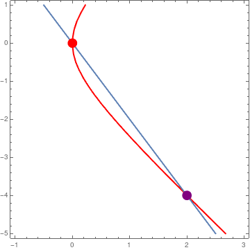
Example 1: The equilibrium points of the nonlinear planar system
|
The x-nullcline is a parabola 4 x = y² - 2 x², and y-nullcline is the straight line y = −2 x. Their intersection consists of two stationary points: the origin (0,0) and (2,−4).
n1 = ContourPlot[4*x - y^2 + 2*x^2 == 0, {x, -1, 3}, {y, -5, 1},
ClippingStyle -> Automatic, ColorFunction -> Hue,
ContourStyle -> Thick];
n2 = ContourPlot[2*x + y == 0, {x, -1, 3}, {y, -5, 1}, ClippingStyle -> Automatic, ColorFunction -> Black, ContourStyle -> Thick]; point = Graphics[{PointSize[0.04], Point[{{0, 0}, {2, -4}}, VertexColors -> {Red, Purple}]}]; Show[n1, n2, point] |
|
| Figure 1: Intersections of two nullclines. | Mathematica code |
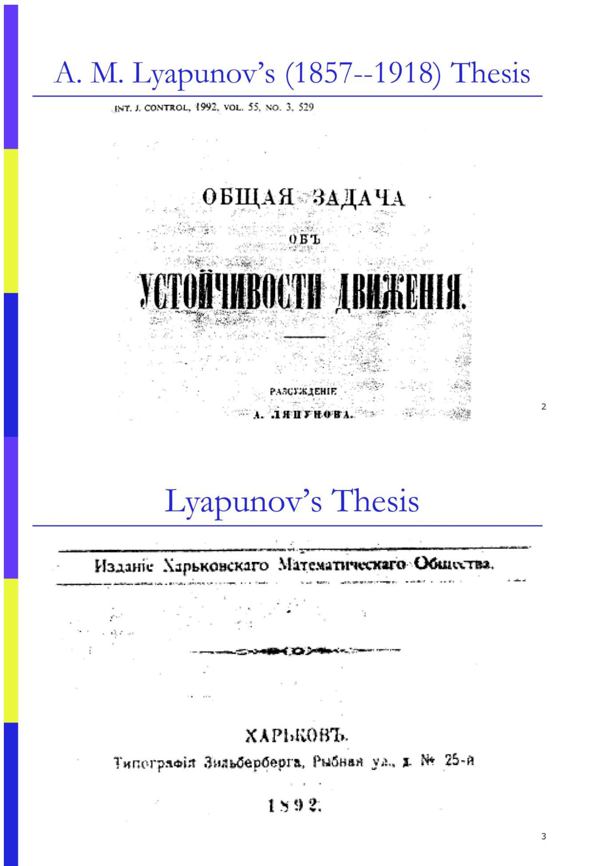
The theory of stability was introduced and further developed by the celebrated Russian mathematician Alexandr Lyapunov (also Liapunov) in 1892. His monograph, entitled: The General Problem of the Stability of Motion, includes so many fruitful ideas and results of primary significance that the whole theory of stability can be divided into two periods, viz. Pre-Lyapunov period and Post-Lyapunov periods.
First of all Lyapunov provided a rigorous definition of motion stability. The absence of such a definition had often caused misunderstandings since otherwise a motion which is stable in one sense can be unstable in another. Then he suggested two main methods for analyzing the stability problems of motions. Of these, the second method, also called The Direct Lyapunov Method is widely popular due to its simplicity and efficiency
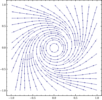
Example 2: Consider the nonlinear system of differential equations \[ \dot{x} = -y + x \left( x^2 + y^2 \right) , \qquad \dot{y} = x + y \left( x^2 + y^2 \right) . \]
|
Upon plotting the phase portrait, we see that the origin is a stable critical point.
sp = StreamPlot[{-y + x*(x^2 + y^2), x + y*(x^2 + y^2)}, {x, -1,
1}, {y, -1, 1}, PerformanceGoal -> "Quality", StreamPoints -> 35,
PlotTheme -> "Classic"]
|
|
| Figure 1: Phase portrait. | Mathematica code |
■
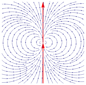
Example: Consider the nonlinear autonomous system of equations
|
sp=StreamPlot[{2*x*y, y^2 - x^2}, {x, -1, 1}, {y, -1, 1},
PerformanceGoal -> "Quality", PlotTheme -> "Classic"];
Introducing polar coordinates
ar = Graphics[{Red, Thickness[0.008], Arrowheads[0.07], Arrow[{{0, -1}, {0, 0}}]}]; line = Graphics[{Red, Thickness[0.008], Arrowheads[0.07], Arrow[{{0, 0}, {0, 1}}]}]; Show[line, ar, sp]
\[
x= t\,\cos\theta , \qquad y = r\,\sin\theta ,
\]
we obtain
\[
\dot{r} = r^2 \sin\theta , \qquad \dot{\theta} = -r\,\cos\theta .
\]
We derive the separable equation
\[
\frac{{\text d}r}{{\text d}\theta} = \frac{\dot{r}}{\dot{\theta}} = -r\,\tan\theta \qquad \left( \theta \ne \frac{\pi}{2} , \quad \theta \ne \frac{3\pi}{2} \right) .
\]
|
|
| Figure 1: Phase portrait. | Mathematica code |
The solution of the latter becomes
Example: ■
An important generalization of the previous definition is uniform asymptotic stability when both of the initial moment t0 and of the initial position x0 of the the perturbed motion do not affect the long-term behavior of the solution.
There are known other definitions of stability (for instance, in Poincaré sense); however, the definitions above (in Lyapunov sense) are mostly used. Before the end of the nineteen century, most of research and applications of differential equations was centered around the analytic expression of solutions of differential equations. Upon the influence of the famous French mathematician Henri Poincaré (1854--1912), the topic of differential equations shifted to the study of the global properties of the solutions without solving the differential equations themselves. The important contributions of Poincaré came at the eve of twentieth century slightly later the Lyapunov discovery. Stability applications have seeped into industry such as in engineering applications, where the common practice is to run a process in “steady state”. For the system that the engineer is interested in, it is frequently of much greater importance to know that the system is approaching a stable equilibrium and will remain there for long time periods, than to have an exact computation of short term transient behavior. Computers make it possible to find approximately the solutions of differential equations on a finite interval of time, but they do not answer the qualitative aspects of the global behavior of phase curves.
A fundamental problem in the theory of differential equations is to study the motion of the system u sing the vector field that induces the differential equations. Qualitative analysis involves questions of the type: Do the solutions go to infinity, or do they remain bounded within a certain region? What conditions must a vector field satisfy in order for the solutions to remain within a given region? Do nearby solutions act similarly to a particular solution of interest? These are questions of qualitative type, in contrast with analytic methods that tend to search for a formula to express each solution of a differential equation. Some authors separate asymptotic stability property when t → ∞ from stability and consider asymptotic stability without requirement for critical point to be stable.
|
x*
A typical quas-asymptotically stable critical point may have the following phase portrait.
c1 = Graphics[{Blue, Thickness[0.01], Circle[{0, 0}, 0.4]}];
c2 = Graphics[{Blue, Thickness[0.01], Circle[{1.6, 0}, {2, 1}]}; c3 = Graphics[{Blue, Thickness[0.01], Circle[{1.3, 0}, {1.7, 0.85}]}]; c4 = Graphics[{Blue, Thickness[0.01], Circle[{1.0, 0}, {1.4, 0.7}]}]; c5 = Graphics[{Blue, Thickness[0.01], Circle[{0.7, 0}, {1.1, 0.55}]}]; Show[c1, c2, c3, c4, c5] |
|
| Quas-asymptotically stable critical point | Mathematica code |
An equilibrium x* is unstable if there exists a positive number ε such that for any δ ≤ ε such that there is at least one solution x = φ(t) that starts within δ-neighborhood of the critical point and be at distance more that ε from the equilibrium solution.
The following (pathological) examples demonstrate that an equilibrium solution can be unstable, but asymptotically stable. This means that there exists a positive number ε such that the magnitude of every nearby solution exceeds it, but eventually all solutions approach the critical point as t → ∞.
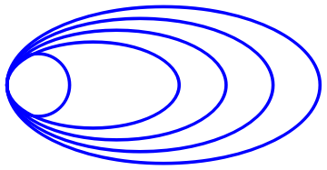
Example: Consider the following system \eqref{EqPlanar.1} due to Thomas Brown (Rassias, J.M., Counter-Examples in Differential Equations, page 95 )
|
circle1 = Graphics[{Thick, Blue, Circle[{0.5, 0.0}, 0.5]}];
circle2 = Graphics[{Thick, Blue, Circle[{1.0, 0.0}, 1.0]}]; arrow1 = Graphics[{Arrowheads[0.04], Blue, Arrow[{{0.98, 0.15}, {1.0, 0}}]}]; arrow2 = Graphics[{Arrowheads[0.045], Blue, Arrow[{{1.98, 0.15}, {2.0, 0}}]}]; circle3 = Graphics[{Thick, Blue, Circle[{1.5, 0.0}, 1.5]}]; arrow3 = Graphics[{Arrowheads[0.045], Blue, Arrow[{{2.98, 0.15}, {3.0, 0}}]}]; c1a = Graphics[{Thick, Blue, Circle[{-0.5, 0.0}, 0.5]}]; a1a = Graphics[{Arrowheads[0.04], Blue, Arrow[{{-0.98, 0.15}, {-1.0, 0}}]}]; c2a = Graphics[{Thick, Blue, Circle[{-1.0, 0.0}, 1.0]}]; a2a = Graphics[{Arrowheads[0.045], Blue, Arrow[{{-1.98, 0.15}, {-2.0, 0}}]}]; c3a = Graphics[{Thick, Blue, Circle[{-1.5, 0.0}, 1.5]}]; a3a = Graphics[{Arrowheads[0.045], Blue, Arrow[{{-2.98, 0.15}, {-3.0, 0}}]}]; c4a = Graphics[{Thick, Blue, Circle[{-2.2, 0.0}, 2.2, {0, -4.5}]}]; c4 = Graphics[{Thick, Blue, Circle[{2.2, 0.0}, 2.2, {-Pi, 1.6}]}]; a4 = Graphics[{Arrowheads[0.05], Blue, Arrow[{{0.32, -1.19}, {0.24, -1.1}}]}]; a4a = Graphics[{Arrowheads[0.05], Blue, Arrow[{{-0.32, -1.19}, {-0.24, -1.1}}]}]; exp = Plot[2.08 + Exp[-x], {x, 0.4, 2.1}, PlotStyle -> {Thick, Blue}]; expa = Plot[2.08 + Exp[x], {x, -2.6, -0.4}, PlotStyle -> {Thick, Blue}]; xa = Graphics[{Arrowheads[0.05], Black, Arrow[{{-4.0, 0}, {5.0, 0}}]}]; xt = Graphics[ Text[StyleForm["x", FontSize -> 18, FontColor -> Black], {4.8, 0.4}]]; ya = Graphics[{Arrowheads[0.05], Black, Arrow[{{0.0, -2.0}, {0.0, 3.7}}]}]; yt = Graphics[ Text[StyleForm["y", FontSize -> 18, FontColor -> Black], {0.4, 3.6}]]; Show[circle1, arrow1, circle2, arrow2, circle3, arrow3, c1a, a1a, c2a, a2a, c3a, a3a, c4, c4a, a4, a4a, exp, expa, ya, yt, xa, xt] |
|
| Some solution trajectories. | Mathematica code |
■
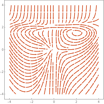
Example: Consider the planar system
|
StreamPlot[{x - y + (x*y - x^3 - x*y^2)/Sqrt[x^2 + y^2],
x + y - (x^2 + y^3 + y*x^2)/Sqrt[x^2 + y^2]}, {x, -2, 2}, {y, -2,
2}, Mesh -> 11, MeshShading -> {Red, None}]
|
|
| Figure 2: Quasi-stable critical point (1,0). | Mathematica code |
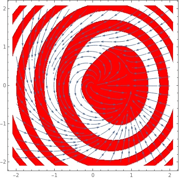
Another unprecedentedly ugly example of quisi-stable system: All solutions nearby 0 goes back to 0, since nearby solutions in the left half plane naturally converge to 0, and nearby solutions in the right half plane first converge to the x-axis, then wind back to the left half plane.
|
StreamPlot[{x^2 + (-(x^2 + 1/16) (y - 1/2)^3) Boole[y >= 1/2], -y + (y - 1)^2 y Boole[y >= 1] - 500 (y - 2)^4 Boole[y >= 2] + (x + 1)^3 Boole[x <= -1] + (x - 1)^3 Boole[x >= 1]}, {x, -4, 4}, {y, -4, 4}, PlotTheme -> "Web"]
|
|
| Figure 3: Quasi-stable critical point (1,0). | Mathematica code |
■
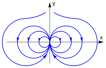
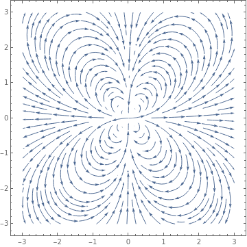
Example: Consider an electric field E given by
Module[{tocartesian, cartesianlist, field, cartesianfield}, tocartesian = {Overscript[r, "^"] -> x/r Overscript[x, "^"] + y/r Overscript[y, "^"], Overscript[\[Theta], "^"] -> -(y/Sqrt[x^2 + y^2]) Overscript[x, "^"] + x/Sqrt[x^2 + y^2] Overscript[y, "^"], r -> Sqrt[x^2 + y^2], \[Theta] -> ArcTan[x, y]};
cartesianlist = (a_ Overscript[x, "^"] + b_ Overscript[y, "^"]) -> {a, b};
field = rfield Overscript[r, "^"] + thetafield Overscript[\[Theta], "^"];
cartesianfield = FullSimplify[field //. tocartesian] /. cartesianlist;
StreamPlot[cartesianfield, opts]]
|
Now we can feed it our original r-θ field definition directly
PolarStreamPlot[{3/(4 r^4) (3 Cos[\[Theta]]^2 - 1),
3/(4 r^4) Sin[2 \[Theta]]}, {x, -3, 3}, {y, -3, 3},
PlotTheme -> "Detailed"]
|
|
| Figure 4: Quasi-stable electric field. | Mathematica code |
|
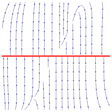
We plot the phase portrait for the given system of nonlinear differential equations
f1[x_, y_] = x^2 *(y - x)*y^5/(x^2 + y^2)/(1 + (x^2 + y^2)^2);
f2[x_, y_] = y^2 *(y - 2*x)/(x^2 + y^2)/(1 + (x^2 + y^2)^2); sp = StreamPlot[{f1[x, y], f2[x, y]}, {x, -1, 1}, {y, -1, 1}, PerformanceGoal -> "Quality", StreamPoints -> 35, PlotTheme -> "Classic"]; line = Graphics[{Red, Thickness[0.01], Line[{{-1, 0}, {1, 0}}]}]; Show[line, sp] |
|
| Figure 1: Phase portrait. | Mathematica code |
■
If every solution of the autonomous system \eqref{EqStability.1} approaches some solution y(t), not necessarily critical point, as t → +∞, then it is called globally asymptotically stable.
The stability of equilibrium solutions of constant coefficient linear systems of differential equations depends completely on the roots of the characteristic polynomial det(λI − A) = 0. The following theorem, credited to the German mathematician Adolf Hurwitz (1859–1919).
Planar Systems
The concepts of asymptotic stability, stability, and instability can be easily visualized by considering two-dimensional models. Let φ(t) = [x(t), y(t)] be the trajectory and x∗ = (x∗, (y∗) be an isolated critical point to the autonomous system. We say that a point P((x, y) approaches he critical point x∗ if \( \lim_{t\to\infty} x(t) = x^{\ast} \) and \( \lim_{t\to\infty} y(t) = y^{\ast} \) ✴
We consider systems of first order ordinary differential equations in normal form on the plane
- Alligood, K.T., Sauer, T.D., and Yorke, J.A., Chaos. An Introduction to Dynamical Systems, 1996, Springer-Verlag, New York, QA614.8.A44 1996
- Cesari, L., Asymptotic Behavior and Stability Problems in Ordinary Differential Equations, Springer-Verlag, Berlin, Heidelberg, 2014. ISBN-13 : 978-3662015308
- Hahn, W. Stability of Motion, Springer-Verlag, Berlin, Heidelberg, 1967.
Return to Mathematica page
Return to the main page (APMA0340)
Return to the Part 1 Matrix Algebra
Return to the Part 2 Linear Systems of Ordinary Differential Equations
Return to the Part 3 Non-linear Systems of Ordinary Differential Equations
Return to the Part 4 Numerical Methods
Return to the Part 5 Fourier Series
Return to the Part 6 Partial Differential Equations
Return to the Part 7 Special Functions