Preface
This section presents basic material about numerical solutions of parabolic equations.
Return to computing page for the first course APMA0330
Return to computing page for the second course APMA0340
Return to Mathematica tutorial for the first course APMA0330
Return to Mathematica tutorial for the second course APMA0340
Return to the main page for the first course APMA0330
Return to the main page for the second course APMA0340
Return to Part VI of the course APMA0340
Introduction to Linear Algebra with Mathematica
Glossary
Numerical Heat Solutions
We demonstrate application of finite difference schemes for numerical solution of the one-dimensional heat equation
Assume that the rectangle \( R= \{\,(x,t)\,:\, 0 \le x \le \ell , \ 0 \le t \le b \,\} \) is subdivided into n-1 and m-1 rectangles with sides Δx = h and Δt = k, as shown in the figure below.
l1 = Graphics[{Thick, Line[{{0, 1}, {8, 1}}]}];
l2 = Graphics[{Thick, Line[{{0, 2}, {8, 2}}]}];
l3 = Graphics[{Thick, Line[{{0, 3}, {8, 3}}]}];
l4 = Graphics[{Thick, Line[{{0, 4}, {8, 4}}]}];
l5 = Graphics[{Thick, Line[{{0, 5}, {8, 5}}]}];
la0 = Graphics[{Thick, Line[{{0, 0}, {0, 6}}]}];
la1 = Graphics[{Thick, Line[{{1, 0}, {1, 6}}]}];
la2 = Graphics[{Thick, Line[{{2, 0}, {2, 6}}]}];
la3 = Graphics[{Thick, Line[{{3, 0}, {3, 6}}]}];
la4 = Graphics[{Thick, Line[{{4, 0}, {4, 6}}]}];
la5 = Graphics[{Thick, Line[{{5, 0}, {5, 6}}]}];
la6 = Graphics[{Thick, Line[{{6, 0}, {6, 6}}]}];
la7 = Graphics[{Thick, Line[{{7, 0}, {7, 6}}]}];
la8 = Graphics[{Thick, Line[{{8, 0}, {8, 6}}]}];
d0 = Graphics[{Orange, Disk[{4, 3}, 0.15]}];
d1 = Graphics[{Orange, Disk[{4, 4}, 0.15]}];
la9 = Graphics[{Thick, Line[{{0, 6}, {8, 6}}]}];
d3 = Graphics[{Orange, Disk[{3, 3}, 0.15]}];
d4 = Graphics[{Orange, Disk[{5, 3}, 0.15]}];
r1 = Graphics[ Text[Style["\!\(\*SubscriptBox[\(x\), \(i\)]\)", Medium], {4, -0.3}]];
r2 = Graphics[Text[ Style["\!\(\*SubscriptBox[\(x\), \(i-1\)]\)", Medium], {3, -0.3}]];
r3 = Graphics[Text[ Style["\!\(\*SubscriptBox[\(x\), \(i+1\)]\)", Medium], {5, -0.3}]];
r4 = Graphics[Text[ Style["\!\(\*SubscriptBox[\(x\), \(n-1\)]\)", Medium], {7, -0.3}]];
r5 = Graphics[Text[ Style["\!\(\*SubscriptBox[\(x\), \(n\)]\)", Medium], {8, -0.3}]];
r6 = Graphics[Text[ Style["\!\(\*SubscriptBox[\(x\), \(2\)]\)", Medium], {1, -0.3}]];
r7 = Graphics[Text[ Style["\!\(\*SubscriptBox[\(x\), \(1\)]\)", Medium], {0, -0.3}]];
t0 = Graphics[Text[ Style["\!\(\*SubscriptBox[\(t\), \(1\)]\)", Medium], {-0.3, 0}]];
t1 = Graphics[Text[ Style["\!\(\*SubscriptBox[\(t\), \(j-1\)]\)", Medium], {-0.4, 2}]];
t2 = Graphics[Text[ Style["\!\(\*SubscriptBox[\(t\), \(j\)]\)", Medium], {-0.3, 3}]];
t3 = Graphics[Text[ Style["\!\(\*SubscriptBox[\(t\), \(j+1\)]\)", Medium], {-0.4, 4}]];
t4 = Graphics[Text[ Style["\!\(\*SubscriptBox[\(t\), \(m\)]\)", Medium], {-0.3, 6}]];
Show[l0, l1, l2, l3, l4, l5, la0, la1, la2, la3, la4, la5, la6, la7, la8, la9, d0, d1, d3, d4, r1, r2, r3, r4, r5, r6, r7, t0, t1, t2, t3, t4]
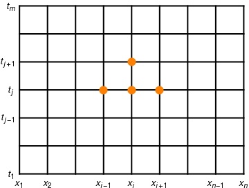
We are going to approximate the solution u(x,t) at grid points in successive rows \( \{ \,u(x_i , t)j )\,:\, i=1,2,\ldots , n \,\} \) for j=2,3,...,m. First, we approximate partial derivatives ut and uxx:
l1 = Graphics[{Thick, Line[{{0, 0}, {0, 2}}]}];
d0 = Graphics[{Red, Disk[{0, 0}, 0.15]}];
d1 = Graphics[{Red, Disk[{4, 0}, 0.15]}];
d2 = Graphics[{Red, Disk[{-4, 0}, 0.15]}];
d3 = Graphics[{Red, Disk[{0, 2}, 0.15]}];
r1 = Graphics[ Text[Style["(1-2r)\!\(\*SubscriptBox[\(u\), \(i,j\)]\)", Medium], {0, -0.5}]];
r2 = Graphics[Text[ Style["r \!\(\*SubscriptBox[\(u\), \(i+1,j\)]\)", Medium], {4.4, -0.3}]];
r3 = Graphics[Text[ Style["r \!\(\*SubscriptBox[\(u\), \(i-1,j\)]\)", Medium], {-4.5, -0.3}]];
r4 = Graphics[Text[ Style["\!\(\*SubscriptBox[\(u\), \(i,j+1\)]\)", Medium], {0, 2.4}]];
Show[l0, l1, d0, d1, d2, d3, r1, r2, r3, r4]
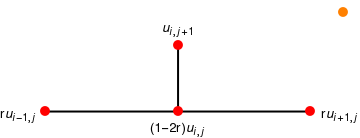
The simplicity of the above formula makes it appealing to use. However, it is important to utilize numerical techniques that are stable. If any error made at one stage of the calculations is eventually dampened out, the method is called stable. The above explicit forward-difference scheme is stable if and only if r is restricted to the interval \( 0 \le r \le \frac{1}{2} . \) This means that the step size k must satisfy so called the Courant--Friedrichs--Lewy or CFL condition: \( k \le h^2 /(2 \alpha^2 ) . \) The condition is named after Richard Courant (1888--1972), Kurt Friedrichs (1901--1982), and Hans Lewy (1904--1988) who described it in their 1928 paper. If the CFL condition is not fulfilled, errors committed in one line { ui,j } might be magnified in subsequent lines { ui,p } for some p > j. The next example illustrates this point.
Example: Consider the initial boundary value problem
For our second illustration, we use the step sizes Δx = h = 0.2 and Δt = k = 0.05, so the ratio becomes r = 1.25. In this case, we get the forward-difference scheme:
Program (Forward-difference method for the heat equation): to approximate the solution of \( u_t = \alpha^2 u_{xx} \) over \( R = \{\,(x,t) \,:\, 0 \le x \le \ell , \ 0 \le t \le b \) with u(x,0) = f(x), for 0 ≤ x ≤ ℓ, and u(0,t) = c0, u(ℓ,t) = cl, for 0 ≤ t ≤ b.
function U=forward(f,c0,cl,a,b,c,n,m)
% Input  -- f=u(x,0) as a string 'f'
%        -- c0=u(0,t) and cl=u(a,t)
%        -- a and b right end points of [0,a] and [0,b]
%        -- c=alpha^2 the thermal diffusivity in heat equation
%        -- n and m number of grid points over [0,a] and [0,b]
% Output -- U solution matrix;
% Initialize parameters and U
h=a/(n-1);
k=b/(m-1);
r=c*k/h^2;
s=1-2*r;
U=zeros(n,m);
% Boundary conditions
U(1,1:m)=c0;
U(n,1:m)=cl;
% Generate the first row
U(2:n-1,1)=feval(f,h:h:(n-2)*h)';
% Generate remaining rows of U
for j=2:m
    for j=2:n-1
        U(i,j)=s*U(i,j-1)+r*(U(i-1,j-1)+U(i+1,j-1));
    end
end
U=U';
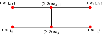
The Crank--Nicholson Method
An implicit finite difference scheme, invented in 1947 by John Crank (1916--2006) and Phyllis Nicholson (1917--1968), is based on numerical approximations for solutions of heat equation at the point (x,t+k/2) and that lies between the rows in the grid. Specifically, the approximation used for ut(x,t+k/2) is obtained from the central-difference formula:
l1 = Graphics[{Thick, Line[{{-4, 2}, {4, 2}}]}];
l2 = Graphics[{Thick, Line[{{0, 0}, {0, 2}}]}];
d0 = Graphics[{Red, Disk[{0, 0}, 0.15]}];
d1 = Graphics[{Red, Disk[{4, 0}, 0.15]}];
d2 = Graphics[{Red, Disk[{-4, 0}, 0.15]}];
d3 = Graphics[{Red, Disk[{0, 2}, 0.15]}];
d4 = Graphics[{Red, Disk[{4, 2}, 0.15]}];
d5 = Graphics[{Red, Disk[{-4, 2}, 0.15]}];
r1 = Graphics[ Text[Style["(2-2r)\!\(\*SubscriptBox[\(u\), \(i,j\)]\)", Medium], {0, -0.5}]];
r2 = Graphics[Text[ Style["r \!\(\*SubscriptBox[\(u\), \(i+1,j\)]\)", Medium], {4.4, -0.3}]];
r3 = Graphics[Text[ Style["r \!\(\*SubscriptBox[\(u\), \(i-1,j\)]\)", Medium], {-4.5, -0.3}]];
r4 = Graphics[Text[ Style["(2+2r)\!\(\*SubscriptBox[\(u\), \(i,j+1\)]\)", Medium], {0, 2.4}]];
r5 = Graphics[Text[ Style["r \!\(\*SubscriptBox[\(u\), \(i-1,j+1\)]\)", Medium], {-4.5, 2.5}]];
r6 = Graphics[Text[ Style["r \!\(\*SubscriptBox[\(u\), \(i+1,j+1\)]\)", Medium], {4.5, 2.5}]];
Show[l0, l1, l2, d0, d1, d2, d3, d4, d5, r1, r2, r3, r4, r5, r6]
Program (Crank--Nicholson method for heat equation): to approximate the solution of \( u_t = \alpha^2 u_{xx} \) over \( R = \{\,(x,t) \,:\, 0 \le x \le \ell , \ 0 \le t \le b \) with u(x,0) = f(x), for 0 ≤ x ≤ ℓ, and u(0,t) = c0, u(ℓ,t) = cl, for 0 ≤ t ≤ b.
function U=crnich(f,c0,cl,a,b,c,n,m)
% Input  -- f=u(x,0) as a string 'f'
%        -- c0=u(0,t) and cl=u(a,t)
%        -- a and b right end points of [0,a] and [0,b]
%        -- c=alpha^2 the thermal diffusivity in heat equation
%        -- n and m number of grid points over [0,a] and [0,b]
% Output -- U solution matrix;
% Initialize parameters and U
h=a/(n-1);
k=b/(m-1);
r=c*k/h^2;
s1=2+2/r;
s2=2/r-2;
U=zeros(n,m);
% Boundary conditions
U(1,1:m)=c0;
U(n,1:m)=cl;
% Generate the first row
U(2:n-1,1)=feval(f,h:h:(n-2)*h)';
% Form the diagonal and off-diagonal elements of A and
% the constant vector B and solve trigiagonal system AX=B
Vd(1,1:n)=s1*ones(1,n);
Vd(n)=1;
Vd(1)=1;
Va=-ones(1,n-1);
Va(n-1)=0;
Vc=-ones(1,n-1);
Vc(1)=0;
Vb(1)=c1;
Vb(n)=c2;
for j=2:m
    for i=2:n-1
        Vb(i)=U(i-1,j-1)+U(i+1,j-1)+s2*U(i,j-1);
    end
    X=trisys(Va,Vd,Vc,Vb);
    U(1:n,j)=X';
end
U=U'
Example: Consider the initial boundary value problem
Other Heat Transfer Equations
Nonlinear Diffusion Equations
Example: Consider the coupled Burgers equations
Example: Consider the coupled Burgers equations ■
- Crank, J. and Nicolson, P. (1947). "A practical method for numerical evaluation of solutions of partial differential equations of the heat conduction type," Proceedings of the Cambridge Philosophical Society, Vol. 43, No. 1, pp. 50--67. doi:10.1007/BF02127704
- Mark Davis, Finite Difference Methods, Imperial College London
- Stability of Finite Difference Methods, http://web.mit.edu/16.90/BackUp/www/pdfs/Chapter14.pdf
Return to Mathematica page
Return to the main page (APMA0340)
Return to the Part 1 Matrix Algebra
Return to the Part 2 Linear Systems of Ordinary Differential Equations
Return to the Part 3 Non-linear Systems of Ordinary Differential Equations
Return to the Part 4 Numerical Methods
Return to the Part 5 Fourier Series
Return to the Part 6 Partial Differential Equations
Return to the Part 7 Special Functions