Preface
This section studies some first order nonlinear ordinary differential equations describing the time evolution (or “motion”) of those hamiltonian systems provided with a first integral linking implicitly both variables to a motion constant. An application has been performed on the Lotka--Volterra predator-prey system, turning to a strongly nonlinear differential equation in the phase variables.
Return to computing page for the first course APMA0330
Return to computing page for the second course APMA0340
Return to Mathematica tutorial for the first course APMA0330
Return to Mathematica tutorial for the second course APMA0340
Return to the main page for the first course APMA0330
Return to the main page for the second course APMA0340
Return to Part III of the course APMA0340
Introduction to Linear Algebra with Mathematica
Glossary
Predator-Prey Equations
Some situations require more than one differential equation to model a particular situation. We might use a system of differential equations to model two interacting species, say where one species preys on the other. For example, we can model how the population of Canadian lynx (lynx Canadians) interacts with a the population of snowshoe hare (lepus americanis) (see https://www.youtube.com/watch?v=ZWucOrSOdCs).
A good historical data are known for the populations of the lynx and snowshoe hare from the Hudson Bay Company. This large Canadian retail company, which owns and operates a large number of retail stores in North America and Europe, including Galeria Kaufhof, Hudson's Bay, Home Outfitters, Lord & Taylor, and Saks Fifth Avenue, was originally founded in 1670 as a fur trading company. The Hudson Bay Company kept accurate records on the number of lynx pelts that were bought from trappers from 1821 to 1940. The company noticed that the number of pelts varied from year to year and that the number of lynx pelts reached a peak about every ten years. The ten year cycle for lynx can be best understood using a system of differential equations.
The primary prey for the Canadian lynx is the snowshoe hare. We will denote the population of hares by H(t) and the population of lynx by L(t), where t is the time measured in years. We will make the following assumptions for our predator-prey model.
- If no lynx are present, we will assume that the hares reproduce at a rate proportional to their population and are not affected by overcrowding. That is, the hare population will grow exponentially,
\[ \frac{{\text d}H}{{\text d}t} = a\,H \qquad (\mbox{where $a$ is a constant}). \]
- Since the lynx prey on the hares, we can argue that the rate at which the hares are consumed by the lynx is proportional to the rate at which the hares and lynx interact. Thus, the equation that predicts the rate of change of the hare population becomes
\[ \frac{{\text d}H}{{\text d}t} = a\,H -b\, H\, L ,\qquad (\mbox{where $a$, $b$ are constants}). \]We are thinking of H L as the number of possible interactions between the lynx and the hare populations.
- If there is no food, the lynx population will decline at a rate proportional to itself,
\[ \frac{{\text d}L}{{\text d}t} = \delta\,L \qquad (\mbox{where $\delta$ is a constant}). \]
- The lynx receive benefit from the hare population. The rate at which lynx are born is proportional to the number of hares that are eaten, and this is proportional to the rate at which the hares and lynx interact. Consequently, the growth rate of the lynx population can be described by
\[ \frac{{\text d}L}{{\text d}t} = c\,H\,L -\delta\, L ,\qquad (\mbox{where $c$, $\delta$ are constants}). \]
The Lotka--Volterra system of equations is an example of a Kolmogorov model, which is a more general framework that can model the dynamics of ecological systems with predator-prey interactions, competition, disease, and mutualism. The equations which model the struggle for existence of two species (prey and predators) bear the name of two scientists: Lotka (1880--1949) and Volterra (1860--1940). They lived in different countries, had distinct professional and life trajectories, but they are linked together by their interest and results in mathematical modeling.
The predator–prey model was initially proposed by Alfred J. Lotka in the theory of autocatalytic chemical reactions in 1910. Lotka was born in Lemberg, Austria-Hungary, but his parents immigrated to the US. In 1925, he utilized the equations to analyze predator-prey interactions. Lotka published almost a hundred articles on various themes in chemistry, physics, epidemiology or biology, about half of them being devoted to population issues. He also wrote six books.
The same set of equations was published in 1926 by Vito Volterra, a mathematician and physicist, who had become interested in mathematical biology because of the impact by the marine biologist Umberto D'Ancona (1896--1964). Vito Volterra was born in Ancona, then part of the Papal States, into a very poor Jewish family. He attended the University of Pisa, where he became professor of rational mechanics in 1883. His most famous work was done on integral equations. In 1892, he became professor of mechanics at the University of Turin and then, in 1900, professor of mathematical physics at the University of Rome La Sapienza. His daughter Luisa married Umberto D’Ancona.
The predator-prey system of equations was later extended by many researchers, including C. S. Holling, Arditi--Ginzburg model, Rosenzweig-McArthur model, and some others.
The critical points of the Lotka--Volterra system of equations are the solutions of the algebraic equations
We may try to find the general solution of the Lotka--Volterra system of equations. From both equations, we get
|
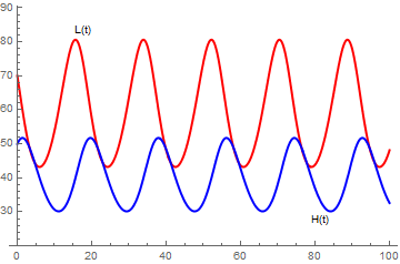
s = NDSolve[{H'[t] == 0.4*H[t] - 0.01*H[t]*L[t],
L'[t] == -0.3*L[t] + 0.005*H[t]*L[t], H[0] == 70, L[0] == 50}, {H, L}, {t, 0, 100}] a = Plot[Evaluate[H[t] /. s], {t, 0, 100}, PlotStyle -> {Thick, Red}, PlotRange -> {20, 85}, PlotLabels -> Placed[{"L(t)"}, Above], PlotLegends -> {"L(t)"}] b = Plot[Evaluate[L[t] /. s], {t, 0, 100}, PlotStyle -> {Thick, Blue}, PlotRange -> {20, 80}, PlotLabels -> Placed[{"H(t)"}, Below], PlotLegends -> {"H(t)"}] Show[{a, b}, PlotRange -> {20, 85}] |
Notice that the predator population, L, begins to grow and reaches a peak after the prey population, H reaches its peak. As the prey population declines, the predator population also declines. Once the predator population is smaller, the prey population has a chance to recover that the cycle begins again.
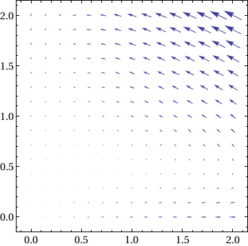
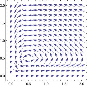
Print["X' = ", MatrixForm[f[x, y]]]
X' = (x-2 x y
-0.5 y+x y )
x' = x-2 x y, y' = -0.5 y+x y
|
Show[VectorPlot[f[x, y], {x, 0, 2}, {y, 0, 2}], Frame -> True,
BaseStyle -> {FontFamily -> "Times", FontSize -> 14}] |
|
Show[VectorPlot[
f[x, y]/(10^-8 + Norm[f[x, y]]), {x, 0, 2}, {y, 0, 2}], Frame -> True, BaseStyle -> {FontFamily -> "Times", FontSize -> 14}] |
|
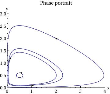
p2 = Show[
ParametricPlot[ Table[{x[t], y[t]} /. sol[[j]], {j, Length[ic]}], {t, 0, T}, PlotRange -> {{0, 4}, {0, 3}}], Table[Graphics[{Arrowheads[.03], Arrow[{ic[[j]], ic[[j]] + .01 f[ic[[j, 1]], ic[[j, 2]] ] }]}], {j, Length[ic]}], AxesLabel -> {"x", "y"}, BaseStyle -> {FontFamily -> "Times", FontSize -> 14}, PlotLabel -> "Phase portrait" ] |
|
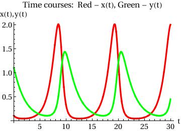
Plot[{x[t] /. sol[[1]], y[t] /. sol[[1]]}, {t, 0, T},
PlotStyle -> {{Thickness[0.01], RGBColor[1, 0, 0]}, {Thickness[0.01], RGBColor[0, 1, 0]}}, AxesOrigin -> {0, 0}, AxesLabel -> {"t", "x(t),y(t)"}, BaseStyle -> {FontFamily -> "Times", FontSize -> 14}, PlotLabel -> "Time courses: Red - x(t), Green - y(t)"] |
we can place two plots sude by side:
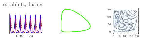
eq1 = r'[t] == a*r[t] - b*r[t]*f[t]
eq2 = f'[t] == -c*f[t] + d*f[t]*r[t]
sol = NDSolve[{eq1, eq2, r[0] == 150, f[0] == 10}, {r, f}, {t, 0, 30}]
gr1 = Plot[Evaluate[{r[t], f[t]} /. sol], {t, 0, 30}, PlotStyle -> {{Thick, Hue[0.7]}, { Dashing[{0.03}], Hue[1]}}, Ticks -> {{{0.01, 0}, {10, "time"}, 20}, {500, {700, "number"}, 1000}}, LabelStyle -> {FontFamily -> "Times", FontSize -> 16}, PlotLabel -> "solid blue: rabbits, dashed red: foxes"];
gr2 = ParametricPlot[Evaluate[{r[t], f[t]} /. sol], {t, 0, 30}, PlotStyle -> {Thick, Hue[0.3]}, Ticks -> {{{0.01`, 0}, 500, {700, "rabbits"}, 1000}, {500, {700, "foxes"}, 1000}}, LabelStyle -> {FontFamily -> "Times", FontSize -> 16}];
sp = StreamPlot[{2.2` r - 0.03 f r, -1.4 f + 0.02` f r}, {r, 0, 200}, {f, 0, 150}, StreamScale -> Large]
GraphicsRow[{gr1, gr2, sp}]
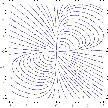 |
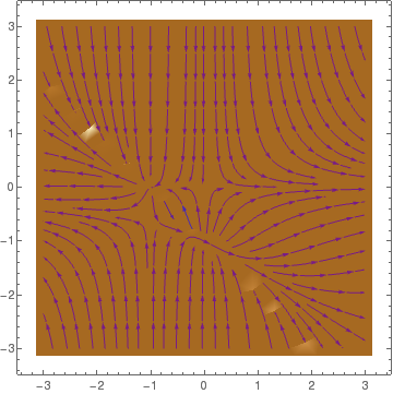
StreamPlot[{x^2 - 3*x*y, 2*x*y - y^2}, {x, -3, 3}, {y, -3, 3}]
|
|
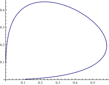
deq1 = x'[t] == x[t]^2 - 3*x[t]*y[t];
Next, we plot the corresponding solutions curve with the command
deq2 = y'[t] == 2*x[t]*y[t] - y[t]^2; soln = NDSolve[{deq1, deq2, x[0] == 1, y[0] == 1}, {x[t], y[t]}, {t, -10, 10}];
x = soln[[1, 1, 2]];
y = soln[[1, 2, 2]];
ParametricPlot[{x, y}, {t, -10, 10}, PlotStyle -> Thick]
|
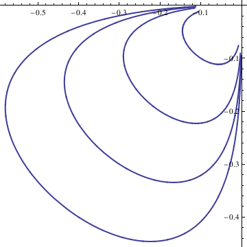 |
curve = Table[n, {n, -4, 4}]; curvep = Table[n, {n, 0, 4}];
Do[Clear[x, y];
soln = NDSolve[{deq1, deq2, x[0] == n/10, y[0] == n/10}, {x[t], y[t]}, {t, -10, 10}]; x = soln[[1, 1, 2]]; y = soln[[1, 2, 2]]; curve[[n]] = ParametricPlot[{x, y}, {t, -10, 10}, PlotStyle -> Thick], {n, -4, 4}]; Show[curve[[-4]], curve[[-3]], curve[[-2]], curve[[-1]], curve[[1]], curve[[2]], curve[[3]], curve[[4]], AspectRatio -> 1] |
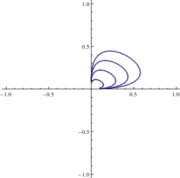 |
Do[Clear[x, y];
soln = NDSolve[{deq1, deq2, x[0] == n/10, y[0] == n/10}, {x[t],
y[t]}, {t, -10, 10}];
x = soln[[1, 1, 2]]; y = soln[[1, 2, 2]]; curvep[[n]] = ParametricPlot[{x, y}, {t, -10, 10}, PlotStyle -> Thick], {n, 0, 4}]; Show[curvep[[0]], curvep[[1]], curvep[[2]], curvep[[3]], curvep[[4]], AspectRatio -> 1] |
- \( \displaystyle 0 < a_1 \delta_1 < K \left( m_1 - \delta_1 \right) \) and
- \( \displaystyle a_2 \delta_2 > K \left( m_2 - \delta_2 \right) \) or \( b_2 \le 1 . \)
Non Kolmogorov models
- The population of prey is sustainable, as they are able to find and have ample food at all times.
- The food supply of predators depends solely on the population of the prey, meaning that the predator eats nothing else but the prey.
- The rate of change of population is proportional to its size.
- The environment is static. It does not change in favor of one species over the other, nor does genetic adaptation play a role.
- The predators’ appetites are limitless.
Thus, we can see that the Lotka-Volterra model fails to impose restrictions on certain parameters, in turn failing to produce realistic projections for predator and prey population data from the field. Two main problems with the Lotka-Volterra model that deter accurate predictions are as follows:
- In the absence of predators (y = 0), the prey population grows exponentially; there is nothing to limit their growth.
- The rate at which predators remove prey is βxy. By dividing this term by y, we see that the rate an individual predator consumes prey is βx. This rate increases as x increases, without any limit for x. Thus, in relation to assumption 5, this implies that an individual predator can never get full.
In order to address the limitations of the Lotka-Volterra model, Rosenzweig and MacArthur proposed their own model in 1963, which more realistically portrays predator-prey interactions.
Mathematical analysis of the Beddington--DeAngelis system shows that there exist two equilibria (0,0) and \( \left( \frac{ac}{ab - b -ac} , \frac{b}{ab - b -ac} \right) = (4,1) , \) being globally stable in the interior of the first quadrant. The eigenvalues of the Jacobian matrix at the origin are \( \lambda_1 =1 \quad\mbox{and}\quad \lambda_2 =5 , \) and the eigenvalues of the Jacobian at the point (4,1) are given by \( - \frac{1}{12} \pm {\bf j} \, \frac{\sqrt{119}}{12} . \)
The Rosenzweig-MacArthur model assumes that the rate at which an individual predator consumes prey has a maximum value:
- M. Rosenzweig and R. MacArthur, Graphical representation and stability con-ditions of predator-prey interaction, American Naturalist (1963) 97, 209-2. https://www.jstor.org/stable/2458702
- Barabas, Gyorgy, D'Andrea, Rafael, and Stump, Simon Maccracken, Chesson's coexistence theory, Ecological Monographs, 2018, https://doi.org/10.1002/ecm.1302
- Batiha, K., Numerical Solutions of the Multispecies Predator-Prey Model by Variational Iteration Method, Journal of Computer Science, 2007, Vol. 3 (7): 523-527, 2007
- Bayliss, A., Nepomnyashchy, A.A., Volpert, V.A., Mathematical modeling of cyclic population dynamics, Physica D: Nonlinear Phenomena, 2019, Volume 394, doi: 10.1016/j.physd.2019.01.010
- Dellal, M., Lakrib, M., Sari, T., The operating diagram of a model of two competitors in a chemostat with an external inhibitor, Mathematical Biosciences, 302, No 8, 2018, 27--45.
- Dimitrov, D.T. and Kojouharov, H.V., Complete mathematical analysis of predator–prey models with linear prey growth and Beddington–DeAngelis functional response, Applied Mathematics and Computation, 162, (2), 523--538, 2005.
- Goel, N.S., Maitra, S.C., and Montroll, E., On the Volterra and other nonlinear models of interacting populations, Reviews of Modern Physics, 1971, Vol. 43, pp. 231-- https://doi.org/10.1103/RevModPhys.43.231
- Hsu, S.B., Hubbell, S.P., and Paul Waltman, Competing predators, SIAM Journal on Applied Mathematics, 35, No 4, 1978, 617--625.
- Hsu, S.B., Hubbell, S.P., and Paul Waltman, A mathematical theory for single-nutrient competition in continuous cultures of micro-organisms, SIAM Journal on Applied Mathematics, Vol 32, No 2, 1977, 366--383.
- Hsu, S.B., Hubbell, S.P., and Paul Waltman, A contribution to the theory of competing predators, Ecological Monographs, Vol 48, No 3, 1978, 337--349.
- May, R.M., Leonard, W.J., Nonlinear Aspects of Competition Between Three Species, SIAM Journal on Applied Mathematics, Vol. 29, Issue 2, pp. https://doi.org/10.1137/0129022
- Molla, H., Rahman, M.S., Sarwardi, S., Dynamics of a Predator–Prey Model with Holling Type II Functional Response Incorporating a Prey Refuge Depending on Both the Species, International Journal of Nonlinear Sciences and Numerical Simulation, 2018, Vol. 20, No. 1, https://doi.org/10.1515/ijnsns-2017-0224
- Olek. S. An accurate solution to the multispecies Lotka-Volterra equations, SIAM Review (Society for Industrial and Applied Mathematics), 1994, Vol. 36(3) (1994), 480–488; https://doi.org/10.1137/1036104
- Ruan, J., Tan, Y., Zhang, C., A Modified Algorithm for Approximate Solutions of Lotka-Volterra systems, Procedia Engineering, 2011, Volume 15, 2011, Pages 1493-1497; https://doi.org/10.1016/j.proeng.2011.08.277
- Scarpello, G.M. and Ritelli, D., A new method for the explicit integration of Lotka--Volterra equations, 2003, Divulgaciones Matematicas, Vol. 11, No. 1, pp. 1--17.
- Seo, Gunog and Wolkowicz, Gail S. K., Sensitivity of the dynamics of the general Rosenzweig--MacArthur model to the mathematical form of the functional response: a bifurcation theory approach. Journal of Mathematical Biology, 76, No 7, 2018, 1873--1906.
Return to Mathematica page
Return to the main page (APMA0340)
Return to the Part 1 Matrix Algebra
Return to the Part 2 Linear Systems of Ordinary Differential Equations
Return to the Part 3 Non-linear Systems of Ordinary Differential Equations
Return to the Part 4 Numerical Methods
Return to the Part 5 Fourier Series
Return to the Part 6 Partial Differential Equations
Return to the Part 7 Special Functions