Preface


This section studies some first order nonlinear ordinary differential equations describing the time evolution (or “motion”) of those hamiltonian systems provided with a first integral linking implicitly both variables to a motion constant. An application has been performed on the Lotka--Volterra predator-prey system, turning to a strongly nonlinear differential equation in the phase variables.

Return to computing page for the first course APMA0330
Return to computing page for the second course APMA0340
Return to Mathematica tutorial for the first course APMA0330
Return to Mathematica tutorial for the second course APMA0340
Return to the main page for the first course APMA0330
Return to the main page for the second course APMA0340
Return to Part III of the course APMA0340
Introduction to Linear Algebra with Mathematica

The Spherical Pendulum


Spherical pendulum.
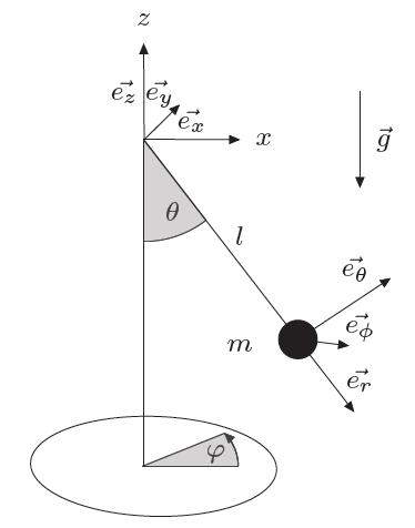
Consider a pendulum bob of mass m hanging from the ceiling by a string of length ℓ and free to move in two dimensions like the Foucault pendulum. This is what is called the spherical pendulum. The free variables are θ and φ of spherical coordinates and the energies are given by
\[ \begin{split} \Pi &= -mg\ell\,\cos\theta , \\ {\mbox K} &= \frac{1}{2}\,m\ell^2 \left( \dot{\theta}^2 + \sin^2 \theta \,\dot{\phi}^2 \right) . \end{split} \]
Then its Lagrangian and Hamiltonian are
\[ \begin{split} L &= {\mbox K} - \Pi = mg\ell\,\cos\theta + \frac{1}{2}\,m\ell^2 \left( \dot{\theta}^2 + \sin^2 \theta \,\dot{\phi}^2 \right) , \\ H &= {\mbox K} + \Pi = -mg\ell\,\cos\theta + \frac{1}{2}\,m\ell^2 \left( \dot{\theta}^2 + \sin^2 \theta \,\dot{\phi}^2 \right) . \end{split} \]
We may calculate the momenta and write the Hamiltonian as a function of them
\[ \begin{split} p_{\phi} &= \frac{\partial H}{\partial \dot{\phi}} = \frac{\partial {\mbox K}}{\partial \dot{\phi}} = m\ell^2 \sin\theta \,\dot{\phi} , \\ p_{\theta} &= \frac{\partial H}{\partial \dot{\theta}} = \frac{\partial {\mbox K}}{\partial \dot{\theta}} = m\ell^2 \dot{\theta} . \end{split} \]
Then the equations of motion become
\[ \begin{split} \dot{p}_{\phi} &= -\frac{\partial H}{\partial \phi} = 0, \\ &\mbox{ showing that angular momentum about the $z$-axis is conserved} \\ \dot{p}_{\theta} &= -\frac{\partial H}{\partial \theta} = \frac{p_{\phi}^2 \cos\theta}{m\ell^2 \sin^3 \theta} - mg\ell\,\sin\theta . \end{split} \]
Note that the Lagrangian is independent of the angular coordinate φ. It follows that \( \sin^2 \theta \,\dot{\phi} \) is a constant. As a result, we get the system of differential equations for the spherical pendulum:
\[ \begin{split} \ddot{\theta} &= \sin\theta\,\cos\theta,\dot{\phi}^2 - \frac{g}{\ell}\,\sin\theta , \\ \frac{\text d}{{\text d}t} \left( \sin^2 \theta \,\dot{\phi} \right) &= 0 \qquad \Longrightarrow \qquad \ddot{\phi} = -2\,\dot{\theta}\dot{\phi}\,\frac{\cos\theta}{\sin\theta} . \end{split} \]
Since \( \sin^2 \theta \,\dot{\phi} = p_{\phi} \) is a constant, we can use the single equation for θ:
\[ \ddot{\theta} = p_{\phi}^2 \,\frac{\cos\theta}{\sin^3 \theta} - \frac{g}{\ell}\,\sin\theta . \]
The total energy is
\[ E = \frac{1}{2} \left( \dot{\theta}^2 + \frac{p_{\phi}^2}{\sin^2 \theta} \right) + \frac{g}{\ell}\,\cos\theta . \]
Let us define an effective potential
\[ U(\theta ) = \frac{1}{2}\, \frac{p_{\phi}^2}{\sin^2 \theta} + \frac{g}{\ell}\,\cos\theta . \]
We define a function for plotting the effective potential, where options may be specified:
effectivePotential[theta0_ /; 0 <= theta0 <= Pi, thetadot0_, phidot0_, opts___Rule] :=
Module[ {pphi}, pphi = (Sin[theta0])^2 phidot0;
Plot[{1/2*(pphi)^2/(Sin[theta])^2 + Cos[theta],
1/2*(thetadot0^2 + (pphi)^2/(Sin[theta0])^2 ) + Cos[theta0] + Cos[theta0]},
{theta, 0 + 10^(-3), Pi - 1/10^3}, Ticks -> {{0, Pi/2, Pi}, Automatic}, AxesLabel -> {"\[Theta]", "U(mgR)"},
PlotStyle -> {{Thickness[0.0075]}, {Dashing[{0.05, 0.05}]}}, opts]]
Now we plot the effective potential:
effectivePotential[2.2, 1.2, -0.1]
The potential function.
For plotting a spherical pendulum, one may us the following code (there is a bug??).
sphericalPendulum[theta0_ /; 0 <= theta0 <= Pi, thetadot0_ /; Abs[thetadot0] < 10, phi0_ /; 0 <= phi0 <= 2*Pi, phidot0_ /; Abs[phidot0] < 10, tmax_ /; 1 <= tmax <= 60, nv_Integer: 999, opts___Rule] := Module[{n = nv, pphi, sol, theta, phi, x, y, z, sphere}, If[n > 1, If[n == 999, n = Round[3 tmax]]; pphi = (Sin[theta0]^2 phidot0 // N); sol = NDSolve[{theta''[t] - Cos[theta[t]]/Sin[theta[t]]^3 + Sin[theta[t]] == 0, phi'[t] == pphi/Sin[theta[t]]^2 , theta[0] = theta0, theta'[0] == thetadot0, phi[0] == phi0}, {theta, phi}, {t, 0, tmax*0.01}, MaxSteps -> 6000]; theta = theta /. First[sol]; phi = phi /. Second[sol]; z[t_] := Cos[theta[t]]; y[t_] := Sin[theta[t]]*Sin[phi[t]]; x[t_] := Sin[theta[t]]*Cos[theta[t]]; sphere = ParametricPlot3D[{{0, Sin[t], Cos[t]}, {Sin[t], 0, Cos[t]}}, {t, 0, 2*Pi}]; ListAnimate[ Table[Show[ sphere, Graphics3D[Line[{{0, 0, -1}, {0, 0, 1}}]], ParametricPlot3D[{x[t], y[t], z[t]}, {t, 0, (tmax/(n - 1))*i + 0.0001}, PlotPoints -> (25 + Round[12*tmax/(n - 1)*i])], Graphics3D[{Thickness[0.0125], Red, Line[{{0, 0, 0}, {x[(tmax/(n - 1))*i], y[(tmax/(n - 1))*i], z[(tmax/(n - 1))*i]}}], PointSize[0.04], Red, Point[{x[(tmax/(n - 1))*i], y[(tmax/(n - 1))*i], z[(tmax/(n - 1))*i]}]}], PlotRange -> {{-1.25, 1.25}, {-1.25, 1.25}}, BoxRatios -> {1, 1, 1}, opts, AxesLabel -> {"x(R)", "y(R)", "z(R)"}], {i, 0, n - 1}]]]]

In rectangular coordinates, the position of the bob and its velocities are

\[ \begin{cases} x&= \ell\,\sin\theta\,\cos\phi , \\ y&= \ell\,\sin\theta\,\sin\phi , \\ z&= -\ell\,\cos\theta ; \end{cases} \qquad\Longrightarrow \qquad \begin{cases} \dot{x}&= \ell\left( \dot{\theta}\,\cos\theta \,\cos\phi - \dot{\phi}\,\sin\theta\,\sin\phi \right) , \\ \dot{y}&= \ell\left( \dot{\theta}\,\sin\theta \,\cos\phi + \dot{\phi}\,\sin\theta\,\cos\phi \right) , \\ \dot{z} &= \ell \dot{\theta}\,\sin\theta . \end{cases} \]
Therefore, the square of the linear velocity is
\[ v^2 = \dot{x}^2 + \dot{y}^2 + \dot{z}^2 = \ell^2 \left( \dot{\theta}^2 + \dot{\phi}^2 \sin^2 \theta \right) . \]
sol = Flatten@ NDSolve[{\[Theta]''[t] == \[Phi]'[t]^2 Cos[\[Theta][t]] -
g/l Sin[\[Theta][t]], \[Phi]''[
t] == (-2 \[Phi]'[t] \[Theta]'[t] Cos[\[Theta][t]])/
Sin[\[Theta][t]], \[Theta][0] == \[Pi]/2, \[Theta]'[0] ==
0, \[Phi][0] == \[Pi]/2, \[Phi]'[0] == 1} /. {g -> 9.81, l -> 1}, {\[Theta], \[Phi]}, {t, 0, 10}]
x[t_] := Evaluate[(Sin[\[Theta][t]] Cos[\[Phi][t]]) /. sol]
y[t_] := Evaluate[(Sin[\[Theta][t]] Sin[\[Phi][t]]) /. sol]
z[t_] := Evaluate[Cos[\[Theta][t]] /. sol]
ParametricPlot3D[{x[t], y[t], z[t]}, {t, 0, 10}]


  1. Arnol'd, V. I. (1989), Mathematical Methods of Classical Mechanics, Springer-Verlag, ISBN 978-0-387-96890-2
  2. Ghorbel, J. and Dabney, J. B., A Spherical Pendulum System to Teach the Concepts in Kinematics, Dynamics, Control, and Simulation, (Aug 19, 2011)


Return to Mathematica page
Return to the main page (APMA0340)
Return to the Part 1 Matrix Algebra
Return to the Part 2 Linear Systems of Ordinary Differential Equations
Return to the Part 3 Non-linear Systems of Ordinary Differential Equations
Return to the Part 4 Numerical Methods
Return to the Part 5 Fourier Series
Return to the Part 6 Partial Differential Equations
Return to the Part 7 Special Functions