Return to computing page for the second course APMA0340
Return to Mathematica tutorial for the second course APMA0340
Return to the main page for the course APMA0330
Return to the main page for the course APMA0340
Return to Part IV of the course APMA0330
Glossary
Pendulum
There are many examples in real life when an object rotates around a particular center. Everyone knows that the planets orbit the Sun in a circular orbit, right? Well ... not exactly. A 17th century mathematician by the name of Johannes Kepler was able to show that the orbits of planets about the sun are elliptical in shape.
For a circular motion, it is convenient to use polar coordinates (r,θ), where r is the distance from the center of rotation and θ is the angle from the reference line, which is usually identified with a positive semi-axis of ordinate in rectangular coordinates. For motion in a circle of radius r, the circumference of the circle is C = 2π r. If the period for one rotation is T, the angular rate of rotation, also known as angular velocity, ω is:
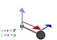
The SI unit for torque is N⋅m. The symbol for torque is typically τ, the lowercase Greek letter τ. In mechanical engineering, it is called moment of force, and is commonly denoted by M. The term torque was introduced into English scientific literature by James Thomson, the brother of Lord Kelvin, in 1884. When force F is applied to a circular rotated object, τ = r × F (with × denoting the cross product). Alternatively,
Taking the derivative, we obtain
The acceleration due to change in the direction is:
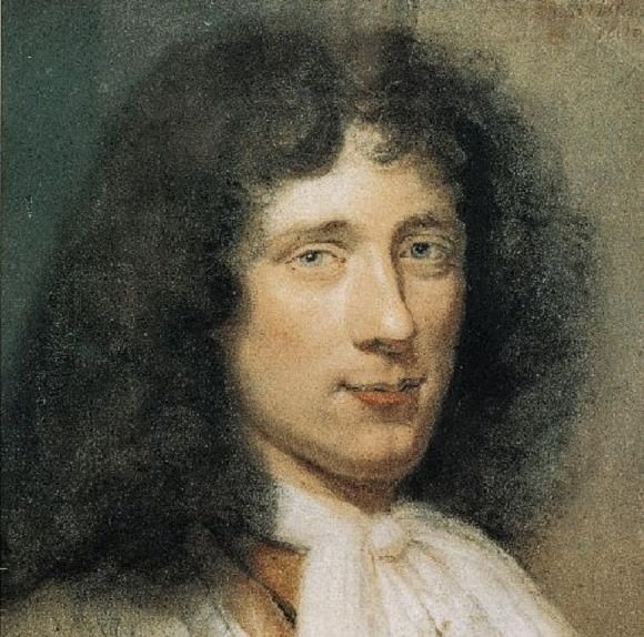
There is no doubt that the first person who investigated and established the mathematical theory and properties of the pendulum was a prominent Dutch mathematician and scientist named Christiaan Huygens (this spelling of his name is taken from the title of his 1658 book Horologium Oscillatorium). The main point of Huygens' (1629--1695) discovery was that the curve in which a pendulum particle (or bob) hangs by a string of insensible weight must move in order to be isochronous in its vibrations, and is not a circle, but a cycloid.
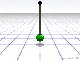
The pendulum consists of a bob (point mass) of mass m attached to the end of a light inextensible rod of length ℓ and negligible weight, with the motion taking place in a vertical plane. Such pendulum is usually referred to as a simple pendulum. Let θ be the angular coordinate of m measured counterclockwise from the down position. We model it as a particle constrained to move in a circle of radius ℓ. Upon choosing rectangular coordinates with the origin at the pivot point and assuming that the pendulum oscillates within the plane, then we label the vertical axis with y so that the pendulum moves in the plane of the circle having the center being the origin. Because the mass must move on the circle, at each time t we have
II. Pendulum Equation with Resistance
IV. Driven Pendulum
A driven pendulum may exhibit a chaotic motion. It consists of a mass m fixed at a distance \( \ell \) from a pivot which is subject to a vertical oscillation \( y = A\, \cos \left( \omega \, t \right) . \) Let θ be the angular coordinate of m measured counterclockwise from the down position, and \( \phi = \pi - \theta \) the complementary displacement measured clockwise from the up orientation. The kinetic and potential energies are
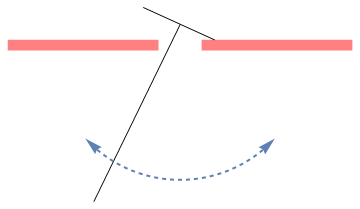
V. Rocking Rigid Pendulum
minus = Polygon[{{1/2, 0}, {1/2, 1/4}, {4, 1/4}, {4, 0}}]
a = Show[Graphics[{Pink, minus}], Graphics[{Pink, plus}]]
line1 = Graphics[Line[{{-2, -3.5}, {0, 0.6}}], PlotRange -> {{-2, 2}, {-4, 1}}]
line2 = Graphics[Line[{{-0.85, 1.0}, {0.8, 0.25}}], PlotRange -> {{-2, 2}, {-4, 1}}]
makeArrowPlot[g_Graphics, ah_: 0.05, dx_: 1*^-6, dy_: 1*^-6] :=
Module[{pr = PlotRange /. Options[g, PlotRange], gg, lhs, rhs},
gg = g /. GraphicsComplex -> (Normal[GraphicsComplex[##]] &);
lhs := Or @@
Flatten[{Thread[Abs[#[[1, 1, 1]] - pr[[1]]] < dx], Thread[Abs[#[[1, 1, 2]] - pr[[2]]] < dy]}] &;
rhs := Or @@ Flatten[{Thread[Abs[#[[1, -1, 1]] - pr[[1]]] < dx], Thread[Abs[#[[1, -1, 2]] - pr[[2]]] < dy]}] &;
gg = gg /.
x_Line?(lhs[#] && rhs[#] &) :> {Arrowheads[{-ah, ah}], Arrow @@ x};
gg = gg /. x_Line?lhs :> {Arrowheads[{-ah, 0}], Arrow @@ x};
gg = gg /. x_Line?rhs :> {Arrowheads[{0, ah}], Arrow @@ x};
gg]
curve = Plot[{-Sqrt[9 - x^2]}, {x, -2.2, 2.2}, PlotStyle -> {Thick, Dashed}, Axes -> False] // makeArrowPlot
Show[a, line1, line2, curve]
minus = Polygon[{{1/2, 0}, {1/2, 1/4}, {4, 1/4}, {4, 0}}]
a = Show[Graphics[{Pink, minus}], Graphics[{Pink, plus}]]
line1 = Graphics[Line[{{-2, -3.5}, {0, 0.6}}], PlotRange -> {{-2, 2}, {-4, 1}}]
line2 = Graphics[Line[{{-0.85, 1.0}, {0.8, 0.25}}], PlotRange -> {{-2, 2}, {-4, 1}}]
p2 = Graphics[{Dashed, Arrow[{{-0.66, -0.8}, {-0.66, -3.8}}]}]
point = Graphics[{PointSize[Large], Green, Point[{-0.66, -0.8
t1 = Graphics[ Text[Style["\[Theta]", FontSize -> 14, Red], {-1.0, -2.4}]]
t2 = Graphics[Text[Style["G", FontSize -> 14, Blue], {-1.0, -0.8}]]
a1 = Graphics[Text[Style["a", FontSize -> 14, Blue], {0.5, 0.7}]]
a2 = Graphics[Text[Style["a", FontSize -> 14, Blue], {-0.2, 1.0}]]
Q = Graphics[Text[Style["Q", FontSize -> 14, Blue], {1.0, 0.45}]]
b = Graphics[Text[Style["b", FontSize -> 14, Blue], {0.0, -0.2}]]
mg = Graphics[Text[Style["mg", FontSize -> 14, Black], {-0.2, -3.6}]]
Show[a, line1, line2, point, p2, t1, t2, a1, a2, Q, b, mg]
minus = Polygon[{{1/2, 0}, {1/2, 1/4}, {4, 1/4}, {4, 0}}]
a = Show[Graphics[{Pink, minus}], Graphics[{Pink, plus}]]
line1 = Graphics[Line[{{2, -3.5}, {0, 0.6}}], PlotRange -> {{-2, 2}, {-4, 1}}]
line2 = Graphics[Line[{{0.85, 1.0}, {-0.8, 0.25}}], PlotRange -> {{-2, 2}, {-4, 1}}]
p2 = Graphics[{Dashed, Arrow[{{0.66, -0.8}, {0.66, -3.8}}]}]
point = Graphics[{PointSize[Large], Green, Point[{0.66, -0.8}]}]
t1 = Graphics[ Text[Style["\[Theta]", FontSize -> 14, Red], {1.0, -2.4}]]
t2 = Graphics[Text[Style["G", FontSize -> 14, Blue], {0.3, -0.8}]]
P = Graphics[Text[Style["P", FontSize -> 14, Blue], {-0.9, 0.45}]]
b = Graphics[Text[Style["b", FontSize -> 14, Blue], {0.0, -0.2}]]
mg = Graphics[Text[Style["mg", FontSize -> 14, Black], {0.22, -3.6}]]
Show[a, line1, line2, point, p2, t1, t2, P, b, mg]
minus = Polygon[{{1/2, 0}, {1/2, 1/4}, {4, 1/4}, {4, 0}}]
a = Show[Graphics[{Pink, minus}], Graphics[{Pink, plus}]]
line1 = Graphics[Line[{{0, -3.5}, {0, 0.6}}], PlotRange -> {{-2, 2}, {-4, 1}}]
line2 = Graphics[Line[{{0.85, 0.27}, {-0.85, 0.27}}], PlotRange -> {{-2, 2}, {-4, 1}}]
P = Graphics[Text[Style["P", FontSize -> 14, Blue], {0.9, 0.45}]]
Q = Graphics[Text[Style["Q", FontSize -> 14, Blue], {-0.9, 0.45}]]
mg = Graphics[Text[Style["mg", FontSize -> 14, Black], {0.4, -3.6}]]
point = Graphics[{PointSize[Large], Green, Point[{0, -0.8}]}]
t2 = Graphics[Text[Style["G", FontSize -> 14, Blue], {-0.3, -0.8}]]
p3 = Graphics[{Dashed, Line[{{0, -0.8}, {0.85, 0.27}}]}]
b = Graphics[Text[Style["b", FontSize -> 14, Blue], {-0.3, -0.2}]]
a1 = Graphics[Text[Style["a", FontSize -> 14, Blue], {0.3, 0.5}]]
a2 = Graphics[Text[Style["a", FontSize -> 14, Blue], {-0.3, 0.5}]]
ell = ToExpression["\ell", TeXForm]
t3 = Graphics[Text[Style[ell, FontSize -> 14, Black], {0.6, -0.4}]]
Show[a, line1, line2, point, p3, t2, a1, a2, P, Q, b, mg, t3]
 |
 |
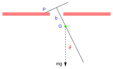 |
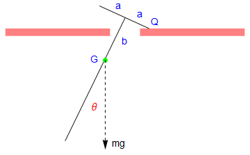
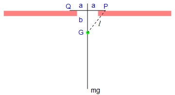
Let the mass of the pendulum be m, and the length of the attached bar be 2 a. Since the construction of the rigid pendulum is symmetric, the center of gyration, which we denote by G, is along the main rod. Let k be the radius of gyration of the pendulum about G, so that the square of its radius of gyration about P and Q is \( k^2 + \ell^2 . \)
The first half-cycle of the motion
Suppose that the pendulum is set in motion from the central position with initial conditions
The first transition through the central position
- Scientific Computing by Jeffrey R. Chasnov.
- Simple Pendulum
- T.H. Fay, The pendulum equation, International Journal of Mathematical Education in Science and Technology, 2002, Vol. 33, No. 4, pp. 505--519.
- Robert A. Nelson and M.G. Olsson, "The pendulum---rich physics from a simple system," American Journal of Physics, 1986, Vol. 54, No 2, 112--121;
- M. G. Olsson, Why does a mass on a spring sometimes misbehave?, American Journal of Physics, 1976, Vol. 54, No. 12, pp. 1211--1212; https://doi.org/10.1119/1.10265
Return to Mathematica page
Return to the main page (APMA0330)
Return to the Part 1 (Plotting)
Return to the Part 2 (First Order ODEs)
Return to the Part 3 (Numerical Methods)
Return to the Part 4 (Second and Higher Order ODEs)
Return to the Part 5 (Series and Recurrences)
Return to the Part 6 (Laplace Transform)
Return to the Part 7 (Boundary Value Problems)