Return to computing page for the second course APMA0340
Return to computing page for the fourth course APMA0360
Return to Mathematica tutorial for the first course APMA0330
Return to Mathematica tutorial for the second course APMA0340
Return to Mathematica tutorial for the fourth course APMA0360
Return to the main page for the course APMA0330
Return to the main page for the course APMA0340
Return to the main page for the course APMA0360
Return to Part I of the course APMA0330
Glossary
Preface
This section addresses a buitiful application of Mathematica to plot figures with fillings. Therefore, this section presents numerous examples.
Plotting with filling
|
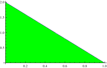
We repeat the previously considered example for a piecewise linear function with filling:
Plot[2 - 2*x, {x, 0, 1}, FillingStyle -> Green, Filling -> Bottom]
|
|
| Piecewise linear function | Mathematica code |
|
Now we change the color of filling:
Plot[2 - 2*x, {x, 0, 1}, FillingStyle -> Green, Filling -> Bottom]
|
|
| Example of green color filling. | Mathematica code |
|
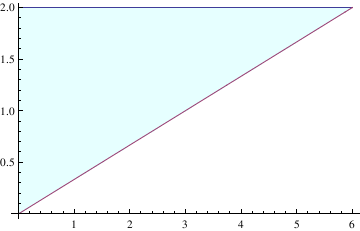
Now we change the color of filling:
Plot[{2, (x/3)}, {x, 0, 6}, Filling -> {1 -> {2}},
FillingStyle -> LightCyan]
|
|
| Example of light cyan color filling. | Mathematica code |
|
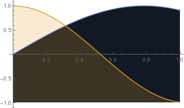
This specifies a specific filling to be used only for the first curve.
Plot[{Sin[2*x], Cos[3*x]}, {x,0,1}, Filling -> {1 -> 0.5}]
|
|
| Two curves with distinct fillings. | Mathematica code |
|
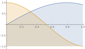
Plot[{Sin[2*x], Cos[3*x]}, {x, 0, 1}, Filling -> Bottom]
|
|
| Region between sine and cosine functions. | Mathematica code |
|
Another color of filling:
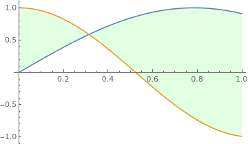
Plot[{Sin[2*x], Cos[3*x]}, {x, 0, 1}, Filling -> {1 -> {2}},
FillingStyle -> LightGreen]
|
|
| Region between sine and cosine functions. | Mathematica code |
|
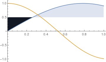
This code specifies a specific filling to be used only for the first curve.
Plot[{Sin[2*x], Cos[3*x]}, {x,0,1}, Filling -> {1 -> 0.5}]
|
|
| Only one part of the region is specified. | Mathematica code |
|
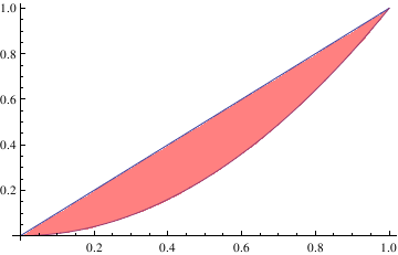
Plot[{x, x^2}, {x, 0, 1}, Filling -> {1 -> {2}}, FillingStyle -> Pink]
|
|
| Region between two curves. | Mathematica code |
|
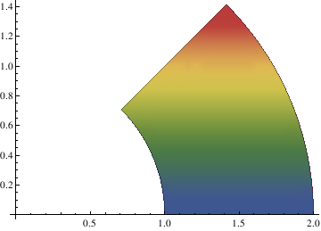
Now we change the color of filling:
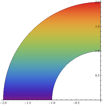
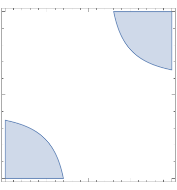
Show[PolarPlot[{1, 2}, {t, 0, Pi/4}],
RegionPlot[
x^2 + y^2 >= 1 && x^2 + y^2 <= 4 && y/x <= 1, {x, 0, 2}, {y, 0, 2},
ColorFunction -> "DarkRainbow"]]
|
|
| Example of PolarPlot. | Mathematica code |
|
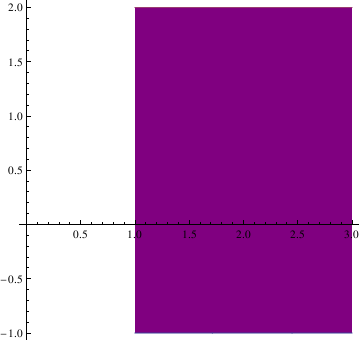
Plot[{-1, 2}, {x, 1, 3}, Filling -> {1 -> {2}},
FillingStyle -> Purple, AspectRatio -> Automatic,
AxesOrigin -> {0, 0}]
|
|
| Rectangle. | Mathematica code |
|
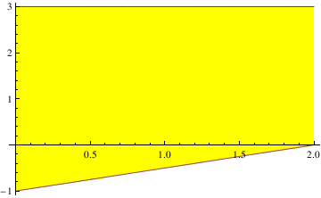
Plot[{3, (x/2) - 1}, {x, 0, 2}, Filling -> {1 -> {2}},
FillingStyle -> Yellow]
|
|
| Figure with filling. | Mathematica code |
|
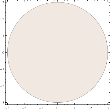
RegionPlot[{x^2 + y^2 <= 9}, {x, -3, 3}, {y, -3, 3},
PlotStyle -> LightBrown]
|
|
| Figure with filling. | Mathematica code |
|
Show[PolarPlot[{1, 2}, {t, Pi/2, Pi}],
RegionPlot[x^2 + y^2 >= 1 && x^2 + y^2 <= 4, {x, -2, 0}, {y, 0, 2},
ColorFunction -> "Rainbow"]]
|
|
| Part of a circle with filling. | Mathematica code |
|
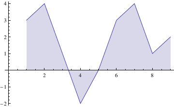
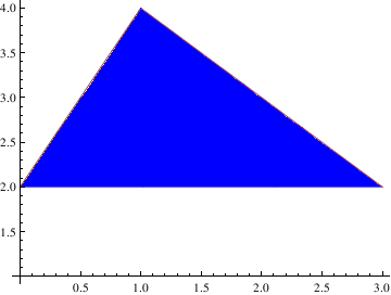
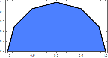
To lift a traingle over the horizontal axis, type:
tr = Plot[{1., Max[1, Min[2 x + 1, 4 - x]]}, {x, 0, 3},
AspectRatio -> 1/2, Ticks -> {{0, 1, 2, 3}, {0, 1, 2, 3}},
Filling -> Axis, FillingStyle -> Blue, Axes -> True, AxesStyle -> Directive[Thick]] a = Graphics[{{Opacity[0], White, tr[[1]]}, GeometricTransformation[{Opacity[1], Blue, tr[[1]]}, TranslationTransform[{0, 1}]]}] Show[a, Axes -> True, AxesStyle -> Black, AspectRatio -> 0.75] |
|
| Triangle is lifted over the axis. | Mathematica code |
FrameTicksStyle -> Directive[FontOpacity -> 0, FontSize -> 0]]
newticks[[All, All, 2]] = "";
 |
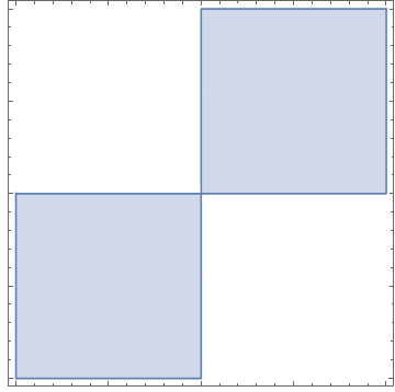
Another example:
Graphics3D[{Texture[img], EdgeForm[],
Cylinder[{{0, 0, 0}, {0, 0, 2 Pi}}, 1]}, Boxed -> False]
|
|
| Two pieces of a circle. | Mathematica code |
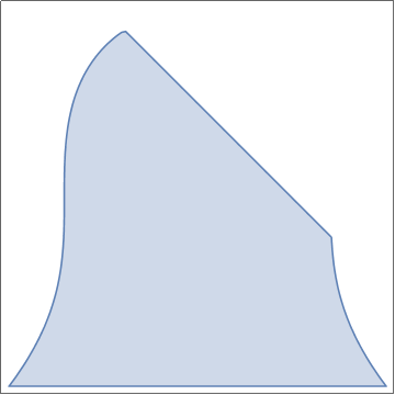
We plot half of the polygon:
Graphics[{RGBColor[0.3, 0.5, 1], EdgeForm[Thickness[0.01]], poly}]
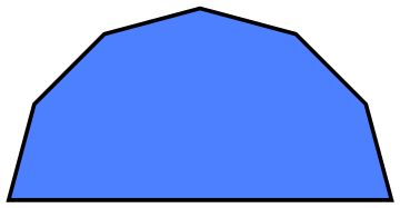
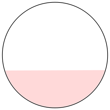 |
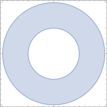
ill = Graphics[{LightRed,
Polygon[Table[{0.99 Cos[theta], 0.99 Sin[theta]}, {theta,
Pi + 0.3, 2 Pi - 0.25, 0.05}]]}];
circle = Graphics[{Black, Thick, Circle[{0, 0}, 1.0]}]; Show[circle, fill] |
|
| Circle with inclusion. | Mathematica code |
Parametric Plots with fillings
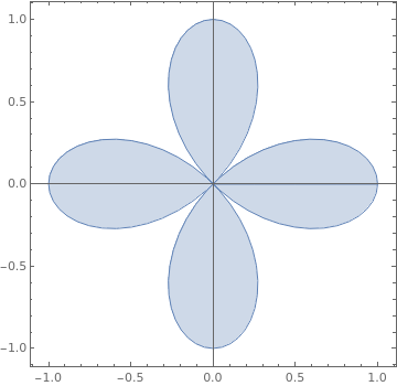 |
ParametricPlot[
Cos[2 theta] {Cos[theta], Sin[theta]} r, {theta, 0, 2 Pi}, {r, 0, 1},
Mesh -> False, PlotPoints -> {30, 2}]
|
|
| Four cusp curve r = cos(2 θ). | Mathematica code |
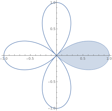 |
g1 = PolarPlot[Cos[2 theta], {theta, Pi/4, 2 Pi - Pi/4}];
g2 = ParametricPlot[ Cos[2 theta] {Cos[theta], Sin[theta]} r, {theta, -Pi/4, Pi/4}, {r, 0, 1}, Mesh -> False]; Show[g1, g2, PlotRange -> All] |
|
| Part of the curve r = cos(2 θ). | Mathematica code |
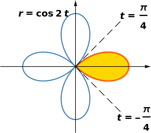 |
txt[t_, {x_, y_}] :=
Style[Text[t, {x, y}], FontSize -> 30, FontWeight -> Bold]
{xmin, xmax} = {-1.425, 1.425}; {ymin, ymax} = {-1.25, 1.25};
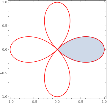
PolarPlot[Cos[2 t], {t, 0, 2 Pi}, PlotRange -> {{xmin, xmax}, {ymin, ymax}}, PlotStyle -> {ColorData["Legacy", "SteelBlue"], Thickness[0.007]}, Ticks -> None, Epilog -> {Inset[ RegionPlot[(x^2 + y^2)^(3/2) <= x^2 - y^2, {x, -0.02, 1}, {y, -1, 1}, PlotStyle -> ColorData["HTML", "Gold"], BoundaryStyle -> Directive[Thickness[0.025], ColorData["Legacy", "CadmiumOrange"]], Frame -> False, AspectRatio -> Automatic, ImageSize -> 2.6*72], {0.5, 0}], Black, Thick, Dashing[{0.045, 0.03}], Line[{{0, 0}, {0.85, 0.85}}], Line[{{0, 0}, {0.85, -0.85}}], Dashing[{}], Thick, Arrow[{{xmin, 0}, {xmax, 0}}], Arrow[{{0, ymin}, {0, ymax}}], txt[TraditionalForm[HoldForm[r == cos 2 t]], {-0.6, 1.0}], txt[TraditionalForm[HoldForm[t == Pi/4]], {1.125, 0.925}], txt[TraditionalForm[HoldForm[t == -Pi/4]], {1.125, -0.99}]}, ImageSize -> 7*72] |
|
| One cusp from the curve r = cos(2 θ). | Mathematica code |
 |
Another version:
Show[{RegionPlot[(x^2 + y^2)^(1/2) <= Cos[2 ArcTan[y/x]], {x, 0,
1}, {y, -1/2, 1/2}],
PolarPlot[Cos[2 theta], {theta, 0, 2 Pi}, PlotStyle -> Red]},
PlotRange -> All]
or
Show[{RegionPlot[(x^2 + y^2)^(3/2) <= x^2 - y^2, {x, 0, 1}, {y, -1/2,
1/2}], PolarPlot[Cos[2 theta], {theta, 0, 2 Pi},
PlotStyle -> Red]}, PlotRange -> All]
or
PolarPlot[Cos[2 theta], {theta, 0, 2 Pi}, PlotStyle -> Red,
Prolog ->
RegionPlot[(x^2 + y^2)^(3/2) <= x^2 - y^2, {x, 0, 1}, {y, -1/2,
1/2}][[1]]]
or
s = PolarPlot[Cos[2 theta], {theta, 0, 2 Pi}];
s1 = PolarPlot[Cos[2 theta], {theta, -Pi/4, Pi/4}] /. Line -> Polygon; Show[s, s1] |
|
| One cusp from the curve r = cos(2 θ). | Mathematica code |
Polar plots with fillings
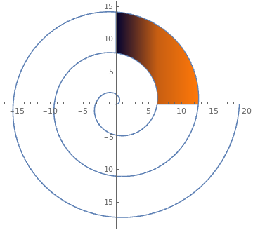 |
parmplot =
ParametricPlot[
r {Cos[t], Sin[t]}, {t, 0, Pi/2}, {r, 2 Pi + t, 4 Pi + t},
ColorFunction -> "RustTones"];
Show[ParametricPlot[t {Cos[t], Sin[t]}, {t, 0, 6 Pi}], parmplot] |
|
| Archimede's spiral. | Mathematica code |
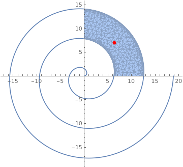 |
cartreg =
ImplicitRegion[
2 \[Pi] < Sqrt[x^2 + y^2] - ArcTan[x, y] < 4 \[Pi] &&
0 <= x <= 15 && 0 <= y <= 15, {x, y}];
regiontoplot = DiscretizeRegion[cartreg, AccuracyGoal -> 5]; NumberForm[#, {8, 5}] &@Area[regiontoplot] NumberForm[Integrate[1, {x, y} \[Element] regiontoplot], {8, 5}]; pt = RegionCentroid[regiontoplot]; Show[ParametricPlot[t {Cos[t], Sin[t]}, {t, 0, 6 Pi}], regiontoplot, Graphics[{PointSize[Large], Red, Point[pt]}]] |
|
| Archimede's spiral with a dot. | Mathematica code |
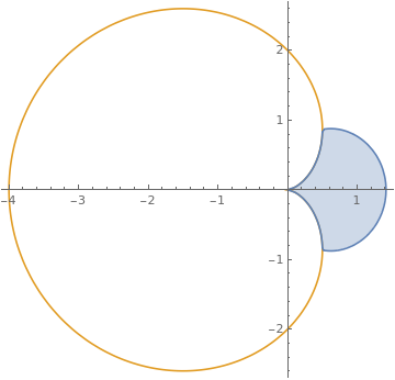 |
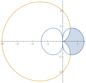
Show[PolarPlot[
Evaluate[{{1, -1} Sqrt[2 Cos[t]],
2 (1 - Cos[t])}], {t, -\[Pi], \[Pi]}],
RegionPlot[
Sqrt[x^2 + y^2] > 2 (1 - Cos[ArcTan[x, y]]) &&
Sqrt[x^2 + y^2] < Re@Sqrt[2 Cos[ArcTan[x, y]]], {x, -2, 2}, {y, -3,
3}], PlotRange -> All]
|
|
| Shading between polar graphs. | Mathematica code |
 |
Another plot:
Show[PolarPlot[{Sqrt[2 Abs[Cos[t]]],
2 (1 - Cos[t])}, {t, -\[Pi], \[Pi]}],
RegionPlot[
4 (1 - Cos[t])^2 < r^2 < 2 Cos[t], {r, 0, 3}, {t, -Pi, Pi},
PlotPoints -> 30] /.
GraphicsComplex[a_, b__] :>
GraphicsComplex[#1 {Cos[#2], Sin[#2]} & @@@ a, b]]
|
|
| Shading between polar graphs. | Mathematica code |
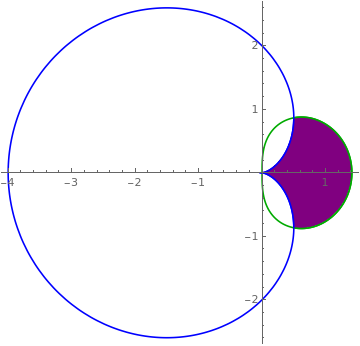 |
Using Cartesian coordinates:
eqns[t_] := {Sqrt[2 Cos[t]], 2 (1 - Cos[t])};
region = PolarPlot[Evaluate@eqns[t], {t, -\[Pi], \[Pi]}, RegionFunction -> Function[{x, y, t, r}, {#1 > #2} & @@ Re[eqns[t]] // First]]; pts = Cases[region, Line[x___] :> x, Infinity]; colors = {Darker@Green, Blue}; Show[PolarPlot[Evaluate@eqns[t], {t, -\[Pi], \[Pi]}, PlotStyle -> colors], ListLinePlot[pts, PlotStyle -> colors, Filling -> Axis, FillingStyle -> Purple], PlotRange -> All] |
|
| Shading between polar graphs. | Mathematica code |
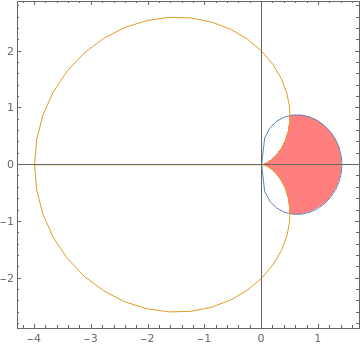 |
You can parameterize your polar functions on to discs, and then shade appropriately.
\[Rho][t_] := Sqrt[2 Cos[t]];
\[Sigma][t_] := 2 (1 - Cos[t]); ParametricPlot[{{r Cos[t] \[Rho][t], r Sin[t] \[Rho][t]}, {r Cos[t] \[Sigma][t], r Sin[t] \[Sigma][t]}}, {t, -\[Pi], \[Pi]}, {r, 0, 1}, PlotStyle -> {{Opacity[.5], Red}, {Opacity[1], White}}, Mesh -> None, PlotRange -> All] |
|
| Shading between polar graphs. | Mathematica code |
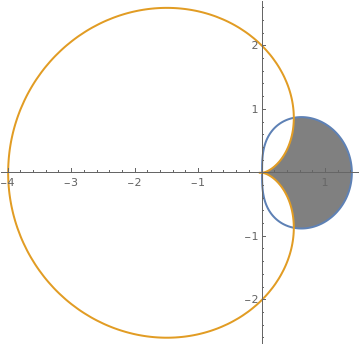 |
Another version:
dt = Pi/99;
pts = Join[ Table[2 (1 - Cos[t]) {Cos[t], Sin[t]}, {t, 0, -Pi/3 + dt, -dt}], Table[Sqrt[2 Cos[t]] {Cos[t], Sin[t]}, {t, -Pi/3, Pi/3, dt}], Table[2 (1 - Cos[t]) {Cos[t], Sin[t]}, {t, Pi/3, dt, -dt}]]; PolarPlot[{Sqrt[2 Cos[t]], 2 (1 - Cos[t])}, {t, -\[Pi], \[Pi]}, Prolog -> {Gray, Polygon[pts]}, PlotStyle -> Thick] |
|
| Shading between polar graphs with contours. | Mathematica code |
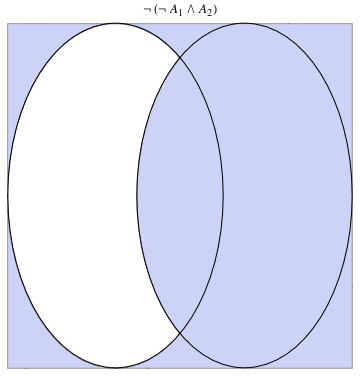
Venn Diagrams
either"directives" or "styles":
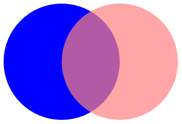
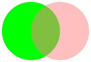
We can plot Venn diagrams using the following subroutine
VennDiagram2[n_, ineqs_: {}] :=
Module[{i, r = .6, R = 1, v, grouprules, x, y, x1, x2, y1, y2, ve},
v = Table[Circle[r {Cos[#], Sin[#]} &[2 Pi (i - 1)/n], R], {i, n}];
{x1, x2} = {Min[#], Max[#]} &[
Flatten@Replace[v,
Circle[{xx_, yy_}, rr_] :> {xx - rr, xx + rr}, {1}]];
{y1, y2} = {Min[#], Max[#]} &[
Flatten@Replace[v,
Circle[{xx_, yy_}, rr_] :> {yy - rr, yy + rr}, {1}]];
ve[x_, y_, i_] :=
v[[i]] /. Circle[{xx_, yy_}, rr_] :> (x - xx)^2 + (y - yy)^2 < rr^2;
grouprules[x_, y_] =
ineqs /.
Table[With[{is = i}, Subscript[_, is] :> ve[x, y, is]], {i, n}];
Show[If[MatchQ[ineqs, {} | False], {},
RegionPlot[grouprules[x, y], {x, x1, x2}, {y, y1, y2},
Axes -> False]],
Graphics[v],
PlotLabel ->
TraditionalForm[Replace[ineqs, {} | False -> \[EmptySet]]],
Frame -> False]]
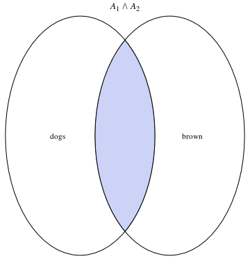
a12 = VennDiagram2[2, Subscript[A, 1] && Subscript[A, 2]]
a1 = Graphics[Text[dogs, {-0.9, 0}]]
b1 = Graphics[Text[brown, {0.9, 0}]]
Show[a12, a1, b1]
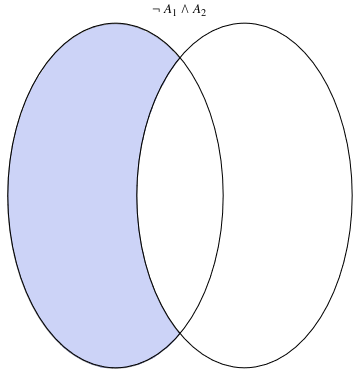
or
a32 = VennDiagram2[2, Not[Subscript[A, 1]] && Subscript[A, 2]]
a33 = VennDiagram2[2, Not[Not[Subscript[A, 1]] && Subscript[A, 2]]]
 |
 |
Return to Mathematica page
Return to the main page (APMA0330)
Return to the Part 1 (Plotting)
Return to the Part 2 (First Order ODEs)
Return to the Part 3 (Numerical Methods)
Return to the Part 4 (Second and Higher Order ODEs)
Return to the Part 5 (Series and Recurrences)
Return to the Part 6 (Laplace Transform)
Return to the Part 7 (Boundary Value Problems)