Return to computing page for the second course APMA0340
Return to Mathematica tutorial for the second course APMA0340
Return to the main page for the course APMA0330
Return to the main page for the course APMA0340
Return to Part IV of the course APMA0330
Glossary
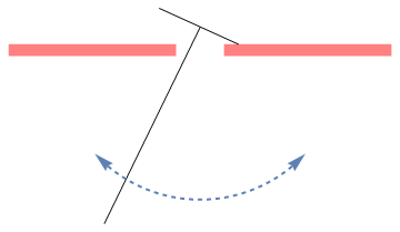
Rocking Pendulum
minus = Polygon[{{1/2, 0}, {1/2, 1/4}, {4, 1/4}, {4, 0}}]
a = Show[Graphics[{Pink, minus}], Graphics[{Pink, plus}]]
line1 = Graphics[Line[{{-2, -3.5}, {0, 0.6}}], PlotRange -> {{-2, 2}, {-4, 1}}]
line2 = Graphics[Line[{{-0.85, 1.0}, {0.8, 0.25}}], PlotRange -> {{-2, 2}, {-4, 1}}]
makeArrowPlot[g_Graphics, ah_: 0.05, dx_: 1*^-6, dy_: 1*^-6] :=
Module[{pr = PlotRange /. Options[g, PlotRange], gg, lhs, rhs},
gg = g /. GraphicsComplex -> (Normal[GraphicsComplex[##]] &);
lhs := Or @@
Flatten[{Thread[Abs[#[[1, 1, 1]] - pr[[1]]] < dx], Thread[Abs[#[[1, 1, 2]] - pr[[2]]] < dy]}] &;
rhs := Or @@ Flatten[{Thread[Abs[#[[1, -1, 1]] - pr[[1]]] < dx], Thread[Abs[#[[1, -1, 2]] - pr[[2]]] < dy]}] &;
gg = gg /.
x_Line?(lhs[#] && rhs[#] &) :> {Arrowheads[{-ah, ah}], Arrow @@ x};
gg = gg /. x_Line?lhs :> {Arrowheads[{-ah, 0}], Arrow @@ x};
gg = gg /. x_Line?rhs :> {Arrowheads[{0, ah}], Arrow @@ x};
gg]
curve = Plot[{-Sqrt[9 - x^2]}, {x, -2.2, 2.2}, PlotStyle -> {Thick, Dashed}, Axes -> False] // makeArrowPlot
Show[a, line1, line2, curve]
minus = Polygon[{{1/2, 0}, {1/2, 1/4}, {4, 1/4}, {4, 0}}]
a = Show[Graphics[{Pink, minus}], Graphics[{Pink, plus}]]
line1 = Graphics[Line[{{-2, -3.5}, {0, 0.6}}], PlotRange -> {{-2, 2}, {-4, 1}}]
line2 = Graphics[Line[{{-0.85, 1.0}, {0.8, 0.25}}], PlotRange -> {{-2, 2}, {-4, 1}}]
p2 = Graphics[{Dashed, Arrow[{{-0.66, -0.8}, {-0.66, -3.8}}]}]
point = Graphics[{PointSize[Large], Green, Point[{-0.66, -0.8
t1 = Graphics[ Text[Style["\[Theta]", FontSize -> 14, Red], {-1.0, -2.4}]]
t2 = Graphics[Text[Style["G", FontSize -> 14, Blue], {-1.0, -0.8}]]
a1 = Graphics[Text[Style["a", FontSize -> 14, Blue], {0.5, 0.7}]]
a2 = Graphics[Text[Style["a", FontSize -> 14, Blue], {-0.2, 1.0}]]
Q = Graphics[Text[Style["Q", FontSize -> 14, Blue], {1.0, 0.45}]]
b = Graphics[Text[Style["b", FontSize -> 14, Blue], {0.0, -0.2}]]
mg = Graphics[Text[Style["mg", FontSize -> 14, Black], {-0.2, -3.6}]]
Show[a, line1, line2, point, p2, t1, t2, a1, a2, Q, b, mg]
minus = Polygon[{{1/2, 0}, {1/2, 1/4}, {4, 1/4}, {4, 0}}]
a = Show[Graphics[{Pink, minus}], Graphics[{Pink, plus}]]
line1 = Graphics[Line[{{2, -3.5}, {0, 0.6}}], PlotRange -> {{-2, 2}, {-4, 1}}]
line2 = Graphics[Line[{{0.85, 1.0}, {-0.8, 0.25}}], PlotRange -> {{-2, 2}, {-4, 1}}]
p2 = Graphics[{Dashed, Arrow[{{0.66, -0.8}, {0.66, -3.8}}]}]
point = Graphics[{PointSize[Large], Green, Point[{0.66, -0.8}]}]
t1 = Graphics[ Text[Style["\[Theta]", FontSize -> 14, Red], {1.0, -2.4}]]
t2 = Graphics[Text[Style["G", FontSize -> 14, Blue], {0.3, -0.8}]]
P = Graphics[Text[Style["P", FontSize -> 14, Blue], {-0.9, 0.45}]]
b = Graphics[Text[Style["b", FontSize -> 14, Blue], {0.0, -0.2}]]
mg = Graphics[Text[Style["mg", FontSize -> 14, Black], {0.22, -3.6}]]
Show[a, line1, line2, point, p2, t1, t2, P, b, mg]
minus = Polygon[{{1/2, 0}, {1/2, 1/4}, {4, 1/4}, {4, 0}}]
a = Show[Graphics[{Pink, minus}], Graphics[{Pink, plus}]]
line1 = Graphics[Line[{{0, -3.5}, {0, 0.6}}], PlotRange -> {{-2, 2}, {-4, 1}}]
line2 = Graphics[Line[{{0.85, 0.27}, {-0.85, 0.27}}], PlotRange -> {{-2, 2}, {-4, 1}}]
P = Graphics[Text[Style["P", FontSize -> 14, Blue], {0.9, 0.45}]]
Q = Graphics[Text[Style["Q", FontSize -> 14, Blue], {-0.9, 0.45}]]
mg = Graphics[Text[Style["mg", FontSize -> 14, Black], {0.4, -3.6}]]
point = Graphics[{PointSize[Large], Green, Point[{0, -0.8}]}]
t2 = Graphics[Text[Style["G", FontSize -> 14, Blue], {-0.3, -0.8}]]
p3 = Graphics[{Dashed, Line[{{0, -0.8}, {0.85, 0.27}}]}]
b = Graphics[Text[Style["b", FontSize -> 14, Blue], {-0.3, -0.2}]]
a1 = Graphics[Text[Style["a", FontSize -> 14, Blue], {0.3, 0.5}]]
a2 = Graphics[Text[Style["a", FontSize -> 14, Blue], {-0.3, 0.5}]]
ell = ToExpression["\ell", TeXForm]
t3 = Graphics[Text[Style[ell, FontSize -> 14, Black], {0.6, -0.4}]]
Show[a, line1, line2, point, p3, t2, a1, a2, P, Q, b, mg, t3]
 |
 |
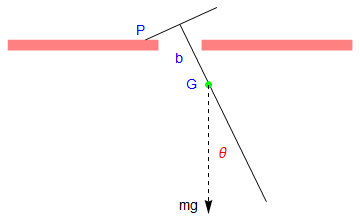 |
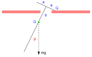
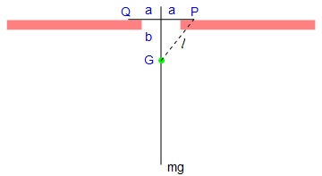
Let the mass of the pendulum be m, and the length of the attached bar be 2 a. Since the construction of the rigid pendulum is symmetric, the center of gyration, which we denote by G, is along the main rod. Let k be the radius of gyration of the pendulum about G, so that the square of its radius of gyration about P and Q is \( k^2 + \ell^2 . \)
The first half-cycle of the motion
Suppose that the pendulum is set in motion from the central position with initial conditions
Return to Mathematica page
Return to the main page (APMA0330)
Return to the Part 1 (Plotting)
Return to the Part 2 (First Order ODEs)
Return to the Part 3 (Numerical Methods)
Return to the Part 4 (Second and Higher Order ODEs)
Return to the Part 5 (Series and Recurrences)
Return to the Part 6 (Laplace Transform)
Return to the Part 7 (Boundary Value Problems)