The set of autonomous equations \( y' = f(y) \) is a subclass of separable differential equations. We discuss some specific properties of these equations.
Return to computing page for the first course APMA0330 Return to computing page for the second course APMA0340 Return to Mathematica tutorial for the first course APMA0330 Return to Mathematica tutorial for the second course APMA0340 Return to the main page for the course APMA0330 Return to the main page for the course APMA0340 Return to Part II of the course APMA0330
where slope function f(y) is a function of only dependent variable and does not involve independent variable explicitly. This equation encompasses, for example, all one-dimensional motions subject to conservative forces,
but also many one-dimensional physical systems. This equation \eqref{EqAuto.1} occurs in cosmology, fluid mechanics, glaciology, hydrology, oceanography, and seismology.
We can make some observations regarding solutions to autonomous equations because their solutions have very limited types of behavior. Their certain mathematical properties are translated into physical properties relevant for natural phenomena. The integral
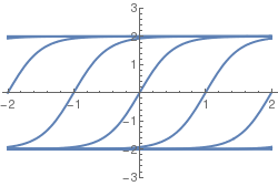
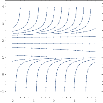
curves (solutions) are invariant under translation along independent variable line, i.e., a horizontal shift of a solution is another solution. For example, consider an autonomous equation
\[ y' = 4 - y^2 . \]
We can plot a family of solutions using Mathematica:
where C is an arbitrary constant. Since the above formula involves the reciprocal of the slope function, we have to exclude from our consideration all points where f vanishes---we have analyses this situation separately.
A point y = y* where \( f\left( y^{\ast} \right) = 0 \) is called a critical point or equilibrium solution for the given differential equation
\( y' = f(y) . \)
Equilibrium solutions can be classified as follows.
Stable: The equilibrium solution y(t) = y* is stable if all solutions with initial condition
y(t0) = y0 "near" the critical point y* approach it as t → ∞. This point is also called a sink.
Unstable: The equilibrium solution y(t) = y* is unstable if all solutions with initial conditions "near" the critical point y* do not approach it as t → ∞.
This point is also called a source.
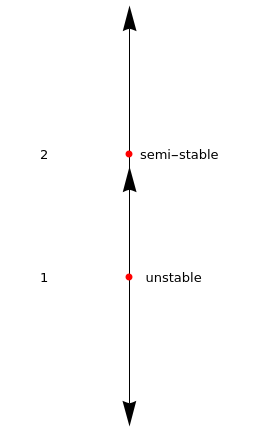
Semi-stable: The equilibrium solution y(t) = y* is semistable if initial conditions y(t0) = y0 "near" the critical point on one side of it lead
to solutions y(t) that approach y* as t → ∞, while initial conditions on the other side of the critical point do not approach it. This point is also called a node.
A critical point is called globally stable if every solution approaches the equilibrium solution independently of the initial conditions.
If the slope function f(x) is continuous, the behavior of solutions of the autonomous equation can be determined from the slope lines along the vertical axis. This leads to construction of what is called a phase line for the differential equation.
Every critical point is a solution of the autonomous differential equation
\( y' = f(y) , \) but solutions cannot cross it. If a solution touches the equilibrium solution, then this stationary solution is a singular solution. According to the existence theorem, if f(y)
and ∂f(y)/ ∂y are continuous in some domain, then in this domain we are guaranteed that no other solution can intersect an equilibrium solution.
The nature of autonomous equations makes spotting constant solutions and interpreting the general behavior of solutions fairly straightforward by analyzing the slope function.
If the slope function is increasing below and decreasing above the critical point ⇒ Stable
If the slope function is decreasing below and increasing above the critical point ⇒ Unstable
If the slope function is decreasing below and above OR increasing below and above ⇒ Semi-stable
Theorem 1: Suppose that the slope function f(y) of the autonomous differential equation \( {\text d}y/{\text d}x = f(y) \) has a continuous derivative
in some interval containing an equilibrium point y*, that is, f(y*) = 0.
If the derivative of f(y) of the slope function evaluated at the critical point is negative, i.e., \( f'\left( y^{\ast} \right) < 0, \) then the equilibrium solution y = y* is stable and the equilibrium solution y* is an attractor. This is a situation when neighbouring solutions that start above with y > y* decrease
toward it, but those neighbouring solutions that start below it with y < y* increase towards the constant solution y*.
If this derivative is positive, that is, \( f'\left( y^{\ast} \right) > 0, \) then the equilibrium solution y = y* is unstable and the critical point is a repellor.
This is a situation when neighbouring solutions that start above with y > y* depart it, but those neighbouring solutions that start below it with y < y* decrease away
from the constant solution y*.
When the derivative of the slope function evaluated at the critical point is zero, \( f'\left( y^{\ast} \right) = 0, \) then the above test is inconclusive. For example, the autonomous differential equation
\[ \dot{y} = f(y) = (y-1)\left( y-2 \right)^2 \]
has two critical points y = 1 (unstable and y = 2 semistable. The derivatives at these points are \( f' (1) = 1 > 0 \) and \( f' (2) = 0 . \)
On the other hand, the differential equation \( \dot{y} = f(y) = (y-1)^3 \) has one unstable critical point y = 1.
Theorem 2: Suppose that the slope function f(y) of the autonomous differential equation \( {\text d}y/{\text d}x = f(y) \) has two continuous derivatives
in some interval containing an equilibrium point y*, at which the slope function has a doublke root: \( f\left( y^{\ast} \right) = f'\left( y^{\ast} \right) = 0 , \quad\mbox{but} \quad f''\left( y^{\ast} \right) \ne 0. \)
If \( f''\left( y^{\ast} \right) < 0, \) then the function f(y) has a maximum at y* and
\( y' = f(y) < 0 \) in neighbourhood of y*. If neighbouring solutions that start below it y < y*, they are running away from it, but neighbouring solutions
that start above it, approach it in phase space. The equilibrium solution is semi-stable.
If \( f''\left( y^{\ast} \right) > 0, \) then the function f(y) has a minimum at y* and
\( y' = f(y) > 0 \) in neighbourhood of y*. The reagion of stability and instability are reversed with respect to the previous case. The equilibrium solution is still semi-stable.
A critical point y = y* of the autonomous differential equation \( y' = f(y) \) is referred to as being hyperbolic if the derivative of the slope function is not zero at the
stationary point:
\( f' \left( y^{\ast} \right) \ne 0 . \) Correspondingly, when \( f' \left( y^{\ast} \right) = 0 \) the case is called nonhyperbolic.
When you observe a higher order root of the slope function f(y), you must look at the lowest order derivative \( f^{(n)} (y) \) that does not vanish at the critical point y*.
If n is odd, the sign of \( f^{(n)} \left( y^{\ast} \right) \) determines stability. So if \( f^{(n)} \left( y^{\ast} \right) < 0,\) it is stable, and if \( f^{(n)} \left( y^{\ast} \right) > 0,\) it is unstable.
If n is even, there is stability on one side and instability on the other side of the constant solution y = y*.
Theorem 3: Let y(x) be a solution of the autonomous differential equation
\( {\text d}y/{\text d}x = f(y) . \) Suppose that the slope function has a continuous derivative in some interval containing an equilibrium point y* and that at some point x0 the solution y(x) enters this interval.
If f(y) > 0 for y(x0) ≤ y < y* or f(y) < 0 for y* < y ≤ y(x0), then \( \lim_{x\to \infty} y(x) = y^{\ast} . \)
If f(y) < 0 for y(x0) ≤ y < y* or f(y) > 0 for y* < y ≤ y(x0), then \( \lim_{x\to -\infty} y(x) = y^{\ast} . \)
Here are three basic examples for illustration of each type of stability:
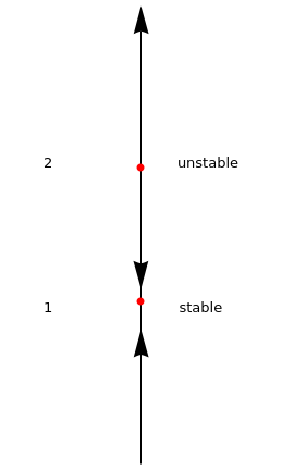
\[ \frac{{\text d}y}{{\text d}t} = \dot{y} = 1- y , \qquad \mbox{critical point $y=1$ is stable}. \]
\[ \dot{y} = y-1 , \qquad \mbox{critical point $y=1$ is unstable}. \]
\[ \dot{y} = \left( 1- y \right)^2 , \qquad \mbox{critical point $y=1$ is semi-stable}. \]
Theorem 4: Let f( y) be a continuous function on the closed interval [𝑎,b] that has only one null y* ∈ (𝑎,b) and f(
y) ≠ 0 for all other points y ∈ ([𝑎,b). If the integral
\[ \int_{y}^{y^\ast} \frac{{\text d}y}{f(y)} \]
diverges, then the initial value problem for the autonomous differential equation \( y' = f(y), \quad y(t_0 ) = y^{\ast} \) has the unique solution y( t) = y*. If the above
integral converges, then the initial value problem has multiple solutions.
Example: We want to find the velocity of the falling parachutist as a function of time t and are particularly interested in the constant limiting velocity, v∞,
due to air resistance. We assume that air drag is proportional to the square of the velocity, -k v², and opposing the force of the gravitational attraction, mg, of the Earth. We choose a coordinate system
in which the positive direction is downward so that the gravitational force is positive. For simplicity we assume that the parachute opens immediately, that is, at time t = 0, where v = 0. Newton’s law applied to
the falling parachutist of total mass m (including chute) gives
where g is the acceleration due to gravity. As usual, the dot indicates the derivative with respect to time variable:
\( \dot{v} = {\text d}v/{\text d}t . \)
The terminal velocity, v∞, can be found from the equation of motion as t → ∞. When there is no acceleration, its velocity is zero, so
where \( \displaystyle s = \sqrt{\frac{m}{k\,g}} \) is the time constant governing the asymptotic approach of the velocity to the limiting velocity v∞. ■
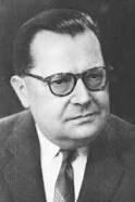
Ludwig von Bertalanffy
Karl Ludwig von Bertalanffy (1901--1972) was an Austrian biologist known as one of the founders of general systems theory. This is an interdisciplinary practice
that describes systems with interacting components, applicable to biology, cybernetics and other fields. He made valuable contributions to the study of organism growth, including the growth of tumors, based on the relationship
between body size of the organism and the metabolic rate. Ludwig theorized that weight is directly proportional to the volume and that the metabolic rate is proportional to surface area. This indicates that surface area is
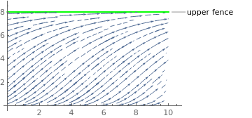
proportional to V2/3 because V is measured in cubic units and its area in square units. Hence, Bertalanffy studied the initial value problem
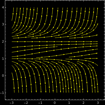
Since the solution approaches (𝑎/b)³ as t → ∞, the horizontal line \( V(t) = (a/b)^3 \) is the upper fence for solutions of the Bertalanffy model. We plot the
corresponding phase portrait:
Example: The bone marrow of a human constantly produces red blood cells (erythrocytes) because they have a finite life span (approximately 120 days). An ordinary differential equations model
of bone marrow erythrocytes was developed in the literature presented below. The model consists of concatenated cell compartments describing the dynamics of the bone marrow cell stages of erythrocytes. Differentiation of cells
is modeled by fluxes from one compartment to the next stage. Proliferation is modeled by amplification in the corresponding compartment. Compartment sizes are modeled by balance equations of the form
where A is the amplification, T is the transit time, C,sup>in is the influx from the previous compartment, and C is the content of the compartment. The oxygen level in kidney tissue determines
the production of erythropoietin (Epo), and the level of Epo is proportional to the rate of red cell production. This means that the oxygen level is inverse proportional to the rate of erythrocyte production. This leads to the
following differential equation model:
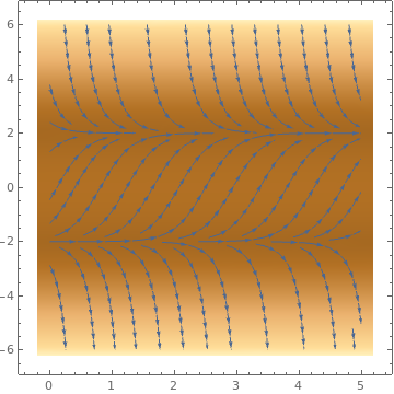
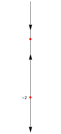
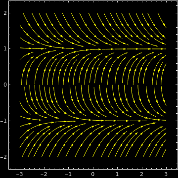
with positive constants 𝑎 and b. This autonomous differential equation has two stable equilibrium solutions (of which only positive one has a physical meaning) y = ±b/𝑎 because the derivative
of the slope function evaluated at these points is negative.
Note that u = 0 corresponds to the vertical line and this point is not a singular point for the red cell model because at this point the differential equation has just horizontal slope:
\[ t + C = \int \frac{u\,{\text d}u}{b - a\,u^2} = -\frac{1}{2a} \int \frac{{\text d} \left( b - a\, u^2 \right)}{b - a\,u^2} = -\frac{1}{2a} \, \ln \left\vert b - a\, u^2 \right\vert , \]
with a constant of integration C. Raising both sides of the above equation to an exponent, we get
\[ b - a\, u^2 = a\,c\, e^{-2a\,t} , \]
with another arbitrary constant c. Hence,
\[ u (t) = \left[ \frac{b}{a} - c\,e^{-2a\,t} \right]^{1/2} \]
is the general solution of the differential equation that serves as a mathematical model of the red cell system.
Loeffler M, Pantel K, Wulff H, Wichmann H (1989) A mathematical model of erythropoiesis in mice and rats. part 1: Structure of the model. Cell Tissue Kinet 22: 13–30.
Pantel K, Loeffler M, Bungart B, Wichmann H (1990) A mathematical model of erythropoiesis in mice and rats. part 4: Differences between bone marrow and spleen. Cell Tissue Kinet 23: 283–297.
Wichmann H (1983) Computer modeling of erythropoiesis. In: Current Concepts in Erythropoiesis, Chapter V., John Wiley and Sons.
Wichmann H, Loeffler M (1985) Mathematical modeling of cell proliferation: Stem cell regulation in hemopoiesis, Vol. 1, 2. CRC Press.
■
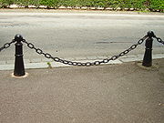
Example: A catenary is the curve that an idealized hanging chain or cable assumes under its own weight when supported only at its
ends. The word "catenary" is derived from the Latin word catēna, which means "chain". The English word "catenary" is usually attributed to Thomas Jefferson. The catenary
is also the surface of revolution, the catenoid, having a minimal surface of revolution.
The mathematical properties of the catenary curve were first studied by Robert Hooke in the 1670s, and its equation was derived by Leibniz,
Huygens, and Johann Bernoulli in 1691.
A chain hanging from points forms a catenary.
Let y(x) be a positive function defined on the interval (x1, x2). Let A(y) be the area of the surface of revolution that we get by rotating the curve y(x)
around the x-axis. From calculus, we know that
Any stationary curve y(x) is a solution of the above nonlinear second order differential equation. Since the above Lagrangian does not explicitly depend on x, we have
Since y(x) is positive, the latter can have a solution only when c1 is negative. Without any loss of generality, we can set α = -c1, where α > 0. Using this,
we have
This is a transcendent equation for α and its solution depends on coordinates of given two points (x1, y1) and (x2, y2). The following cases
are known to occur.
There exists no Catenary connecting the points (x1,y1) and (x2,y2).
There exists exactly one Catenary connecting the points (x1,y1) and (x2,y2).
Milk There exists exactly two Catenaries connecting the points (x1,y1) and (x2,y2).
In case ii) the unique catenary is neither a global nor local minimum. In case iii), one of the solutions is a local minimum, and this is also a global minimum, if y1 is large enough in a certain sense.
Therefore, a surface of revolution of minimum area exists only in case iii) and only if y1 is large enough.
Chain's equation
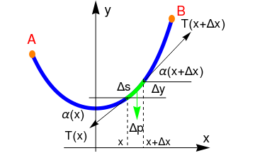
Suppose that a heavy uniform chain is suspended at points Mi>A,B, which may be at different heights (see figure). Consider equilibrium of a small element of the chain of length Δs. The forces acting on
the section of the chain are the distributed force of gravity
where ρ is the density of the chain material, g is the acceleration of gravity, A is the cross sectional area of the thread, and the tension forces T(x) and T(x+Δx),
respectively, at points x and x+Δx.
The equilibrium conditions of the element of the length &Deltas for projections on the axes Ox and Oy are turned out to be
\[ \begin{split} -T\left( x\right) \cos\alpha (x) + T\left( x + \Delta x \right) \cos \alpha (x+\Delta x) &= 0, \\ -T\left( x\right) \sin\alpha (x) + T\left( x + \Delta x \right) \sin \alpha (x+\Delta x) - \Delta P &= 0 \end{split} \]
It follows from the first equation that the horizontal component of the tension force T(x) is always a constant:
Multiplying both sides of the equation by the conjugate expression
\( \displaystyle u - \sqrt{1+u^2} \) gives
\[ \left( u + \sqrt{1+u^2} \right) \left( u - \sqrt{1+u^2} \right) = \left( u - \sqrt{1+u^2} \right)e^{/a} . \]
Upon simplification, we have
\[ u - \sqrt{1+u^2} = e e^{-x/a} . \]
Adding to the previous equation, we find the expression for
\( \displaystyle u = y' : \)
\[ u + \sqrt{1+u^2} + u - \sqrt{1+u^2} = e^{x/a} - e^{-x/a} \qquad \Longrightarrow \qquad u = y' = \sinh \frac{x}{a} . \]
Integrating once more gives the final nice expression for the shape of the catenary:
\[ y = a\,\cosh \frac{x}{a} . \]
The catenary has another interesting feature. When revolved about the x-axis, the catenary gives the surface called catenoid. This surface has minimum surface area,
i.e. any part of the catenoid will be less than any other surface bounded by the same contour. Catenoid was first described in 1744 by the mathematician Leonhard Euler.
In particular, the soap film between two circles trying to minimize the free energy takes the form of a catenoid. ■
\[ \frac{{\text d}y}{(y-1)^2} = {\text d}x \qquad \Longrightarrow \qquad -\frac{1}{y-1} = x + C , \]
we find the general solution in explicit form (which is a very rare case)
\[ y = 1 + \frac{1}{x+C} . \]
To satisfy the initial condition, we are forced to set the arbitrary constant to be infinity and the required solution y = 1. If we make a 1% change in the initial condition to y(0) = 1.01, we obtain a hyperbola
\[ y = 1 + \frac{1}{x-100} , \]
with one vertical asymptote. If we perturb the driving input again by 1%,
with vertical asymptotes at (2n+1)5π, n = 0, ±1, ±2, .... Hence, we see how sensitive a nonlnear differential equation can be to small perturbations.
■
Arino, O. and Kimmel, M., Stability analysis of models of cell production systems, Mathematical Modeling, 1986, Vol. 7, pp. 1269--1300.
Return to Mathematica page Return to the main page (APMA0330) Return to the Part 1 (Plotting) Return to the Part 2 (First Order ODEs) Return to the Part 3 (Numerical Methods) Return to the Part 4 (Second and Higher Order ODEs) Return to the Part 5 (Series and Recurrences) Return to the Part 6 (Laplace Transform) Return to the Part 7 (Boundary Value Problems)