}

Preface


This section gives an introduction to the theory of linear differential operators.

Return to computing page for the first course APMA0330
Return to computing page for the second course APMA0340
Return to Mathematica tutorial for the first course APMA0330
Return to Mathematica tutorial for the second course APMA0340
Return to the main page for the course APMA0330
Return to the main page for the course APMA0340

Linear Operators


Stefan Banach.

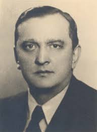
The modern definition of a linear operator was first given by Giuseppe Peano for a particular case. However, it was Stefen Banach who defined an operator as a function whose domain is a set of functions. Stefan Banach (1892 – 1945) was a Polish mathematician who is generally considered one of the world's most important and influential 20th-century mathematicians. He was one of the founders of modern functional analysis, and an original member of the Lwów School of Mathematics. When Nazi German troops conquered Lvov in 1941, all institutions of higher education were closed to Poles. The majority of intelligent people (professors, musicians, actors, writers, painters, and many others) were executed, but Banach survived the Nazi slaughter of Polish university professors. Stefan was born in Kraków (then part of the Austro-Hungarian Empire) and passed away in Lvov (Soviet Union) with lung cancer. Stefan was a heavy smoker, and his name was given to one famous probabilistic problem, as well as to many theorems. From 1910 to 1914 and since 1920, he dwelt in Lvov (Lwów, in Polish). At the time Banach studied there, under Austrian control as it had been from the partition of Poland in 1772. In Banach's youth Poland, in some sense, did not exist and Russia controlled much of the country. Banach was given the surname of his mother, who was identified as Katarzyna Banach on his birth certificate, and the first name of his father, Stefan Greczek. He never knew his mother, who vanished from the scene after Stefan was baptized, when he was only four days old, and nothing more is known of her.

In the spring of 1916, Hugo Steinhaus (1887--1972) made a major impact on Banach's life. Stefan wrote his first paper together with Steinhaus. Banach major work was the 1932 book, Théorie des opérations linéaires (Theory of Linear Operations), the first monograph on the general theory of functional analysis. Hugo Steinhaus was a Polish mathematician (of Jewish decent) whose book Mathematical Snapshots has been very influential. Steinhaus obtained his PhD under David Hilbert.

By an operator we mean a transformation that maps a function into another function. A linear operator L is an operator such that \( L[af+bg] = aLf + bLg \) for any functions f, g and any constants a, b. Since we mostly interested in linear differential operators, we need to start with the derivative operator, which we denote by \( \texttt{D} . \) From calculus, we know that the result of application of the derivative operator on a function is its derivative:

\[ \texttt{D} f (x) = f' (x) = \frac{{\text d}f}{{\text d}x} \qquad \mbox{or, if independent variable is $t$,} \quad \texttt{D} y (t) = \frac{{\text d}y}{{\text d}t} = \dot{y}. \]
We also know that the derivative operator and one of its inverses, \( \texttt{D}^{-1} = \int , \) are both linear operators. It is easy to construct compositions of derivative operator recursively \( \texttt{D}^{n} = \texttt{D} \left( \texttt{D}^{n-1} \right) , \quad n=1,2,\ldots ,\) and their linear combinations:
\begin{equation} \label{EqBanach.1} L\left[ x,\texttt{D} \right] = a_n \texttt{D}^{n} + a_{n-1} \texttt{D}^{n-1} + \cdots a_1 \texttt{D} + a_0 \texttt{I}, \qquad a_n \ne 0, \end{equation}
where coefficients \( a_n , \ a_{n-1} , \ \ldots , \ a_1, \ a_0 , \) of the linear differential operator \( L\left[ x,\texttt{D} \right] \) could be either some functions or even constants. Generally speaking, we should multiply the last coefficient 𝑎0 by the identity operator, \( {\bf I} = \texttt{D}^0 , \) but lazy people usually drop it. Since multiplication by the identity operator does not change the result, we can omit it. The leading coefficient an is assumed to be not identically zero. In this case we say that the linear differential operator is of the order n.

Let us consider, for simplicity, the case n = 2. With a function y = y(x) that is twice differentiable, we assign another function, which we denote (L y)(x) (or L[y] or simply Ly). L[y] is the linear differential operator that acts on y(x) by the relation

\begin{equation} \label{E411.1} (L\,y) (x) % \equiv L[y](x) \equiv Ly(x) = a_2 (x)\,y'' (x) + a_1 (x) y' (x) + a_0 (x) y (x) , \end{equation}
where \( a_2 (x), \ a_1 (x), \ \mbox{ and } a_0 (x) \) are given functions, and \( a_2 (x) \ne 0. \) In mathematical terminology, L is an operator that acts on functions; that is, there is a prescribed recipe for associating with each function y(x) a new function (L y)(x). In other words, an operator L assigns to each function y(x) having two derivatives a new function called (L y)(x). Therefore, the concept of an operator coincides with the concept of a ``function of a function.''

With such defined linear differential operator, we can rewrite any linear differential equation in operator form:

\begin{equation} \label{EqBanach.2} L\left[ x,\texttt{D} \right] y =f(x) \qquad\Longleftrightarrow \qquad \left[ a_n \texttt{D}^{n} + a_{n-1} \texttt{D}^{n-1} + \cdots a_1 \texttt{D} + a_0 \right] y =f(x) \qquad\Longleftrightarrow \qquad a_n y^{(n)} + a_{n-1} y^{(n-1)} + \cdots + a_1 y' + a_0 y = f(x) . \end{equation}
If the right-hand term (also called the driving function) is not identically zero, \( f(x) \ne 0 , \) we call the above equation nonhomogeneous (or inhomogeneous). The equation, which is referred to as the homogeneous equation, with an identically zero driving term is of particular interest:
\begin{equation} \label{EqBanach.3} L\left[ x,\texttt{D} \right] y =0 \qquad\Longleftrightarrow \qquad a_n y^{(n)} + a_{n-1} y^{(n-1)} + \cdots + a_1 y' + a_0 y = 0 . \end{equation}
The set of all solutions of the homogeneous equation \( L\left[ x,\texttt{D} \right] y =0 \) is called the kernel (or nullspace) of the differential operator. In other words, any solution of the above homogeneous linear differential equation belongs to the kernel of the corresponding differential operator.
Example 1: Let \( L\left[ x,\texttt{D} \right] = \texttt{D} - x^2 \) be a first order linear differential operator (with variable coefficient). Find its kernel, denoted by ker(L).

Solution: Let \( y \in \mbox{ker}(L) , \) then by the definition of the kernel,

\[ L\left[ x,\texttt{D} \right] y =0 \qquad\Longleftrightarrow \qquad y' - x^2 y = 0 \qquad\Longleftrightarrow \qquad \frac{{\text d}y}{y} = x^2 {\text d}x . \]

Separating variables and integrating, we obtain
\[ y = C\, e^{x^3 /3} , \]
where C is an arbitrary constant. Therefore, the kernel of the given differential operator consists of all multiples of the exponential function.    ■
Example 2: Consider the second order Chebyshev differential operator of second kind
\[ U_n \left[ x,\texttt{D} \right] = \left( 1 - x^2 \right) \texttt{D}^2 -x\, \texttt{D} + n(n+2) , \qquad x\in (-1,1) , \]
where n is a positive integer and \( \texttt{D} = {\text d}/{\text d}x \) is the derivative operator, that is, \( \texttt{D} y = y' = {\text d}y/{\text d}x \quad\mbox{and}\quad \texttt{D}^2 y = y''. \) The corresponding differential equation
\[ U_n \left[ x,\texttt{D} \right] y \equiv \left( 1 - x^2 \right) y'' -x\, y' + n(n+2)\, y =0 \]
is known to have a polynomial solution \( y= U_n ( x ) , \) called the Chebyshev polynomial of the second kind. Mathematica has a dedicated command to define such polynomial: ChebyshevU[x,n]. We find another linearly independent solution using reduction of order. So we seek another solution in the form

\[ y = u(x)\, U_n (x) \qquad\Longrightarrow \qquad \left( 1 - x^2 \right) u'' U_n + \left( 1 - x^2 \right) u'\,2\,U'_n - x\,u' U_n =0 . \]
Denoting the first derivative of u as v = u', we get the first order separable differential equation
\[ v'(x) + v \, \frac{\left( 1 - x^2 \right) 2 U'_n - x\, U_n}{\left( 1 - x^2 \right) U_n} \qquad\Longrightarrow \qquad \frac{{\text d}v}{v} = \left[ \frac{x}{1-x^2} - 2\, \frac{U'_n}{U_n} \right] {\text d}x . \]
Integration yields
\[ \ln v = -2\,\ln U_n (x) - \frac{1}{2}\,\ln \left( 1- x^2 \right) \qquad\Longrightarrow \qquad v = u' = \frac{C_1}{U_n^2 \left( 1-x^2 \right)^{1/2}} . \]
Next integration gives
\[ u(x) = C_2 + C_1 \int \frac{{\text d}x}{U_n^2 \sqrt{1-x^2}} \]
Therefore, the kernel of the Chebyshev differential operator of the second order is spanned on two functions
\[ U_n (x) \qquad\mbox{and} \qquad U_n (x)\, \int \frac{{\text d}x}{U_n^2 \sqrt{1-x^2}} . \]
   ■
We summarize our observation in the following theorem:

Theorem 1: The kernel of a linear differential operator of order n with continuous coefficients in some interval is n-dimensional and it is spanned on n

linearly independent functions \( y_1 (x), \ y_2 (x), \ \ldots , y_n (x) . \) Then any solution of the homogeneous linear differential equation \( L\left[ x,\texttt{D} \right] y =0 \) can be represented as a linear combination of these functions
\[ y(x) = C_1 y_1 (x) + C_2 y_2 (x) + \cdots + C_n y_n (x) , \]
with some constants C1, ... , Cn    ⧫


Adjoint Operators


In the functional space 𝔏²(𝑎, b) of square-integrable functions on a real interval (𝑎a, b), the scalar product is defined by
\begin{equation} \label{EqAdjoint.1} \left\langle f, g \right\rangle = \int_a^b \overline{f(x)}, g(x) \,{\text d}x , \end{equation}
where the line over f(x) denotes the complex conjugate of f(x). If one moreover adds the condition that f or g vanishes for x → 𝑎 and xb, one can also define the adjoint operator
\begin{equation} \label{EqAdjoint.2} L^{\ast} \left[ x, \texttt{D} \right] = \sum_{k=0}^n (-1)^k \texttt{D}^k \left[ \overline{a_k (x)} \right] , \qquad L \left[ x, \texttt{D} \right] = \sum_{k=0}^n a_k \texttt{D}^k \end{equation}
to the n-order differential operator \eqref{EqBanach.1}. With another inner product, we will get another formular for the adjoint operator. A (formally) self-adjoint operator is an operator equal to its own (formal) adjoint.

For a second order linear differential operator \eqref{EqBanach.2}, correspond the adjoint operator is

\begin{equation} \label{EqAdjoint.3} L^{\ast} \left[ x, \texttt{D} \right] = a_2 (x)\, \texttt{D}^2 + \left( 2a'_2 -a_1 \right) \texttt{D} + \left( a''_2 - a'_1 + a_0 \right)\texttt{D}^0 , \qquad L \left[ x, \texttt{D} \right] = a_2 \texttt{D}^2 + a_1 \texttt{D} + a_0 \texttt{D}^0 . \end{equation}
As usual, primes denote differentiation and \( \texttt{D}^0 = \texttt{I} \) is the identical operator.

Theorem 2: If φ(x) is a solution of a second order homogeneous equation

\[ a_2 (x)\,\varphi'' + a_1 (x)\, \varphi' + a_0 (a) \,\varphi =0 , \]
then the function
\[ \psi (x) = \frac{a_2 (x)}{W[x]} \,\varphi (x) \]
is a solution of the adjoint homogeneous equation
\[ a_2 \psi'' + \left( a''_2 - a'_1 + a_0 \right) \psi' + \left( a''_2 - a'_1 + a_0 \right) \psi = 0 . \]
Here \( W[x] = W \left( x_0 \right) \exp \left\{ -\int a_1 (x)/a_2 (x)\,{\text d}x \right\} \) is the Wronskian (arbitrary multiplier is ommited) of the operator \eqref{EqBanach.2}.    ⧫
Example 3: Consider the differential operator
\[ L\left[ x, \texttt{D} \right] = \texttt{D}^2 + x\, \texttt{D} + x\,\texttt{I} . \]
Its adjoint is
\[ L^{\ast} \left[ x, \texttt{D} \right] = \texttt{D}^2 - x\, \texttt{D} + \left( x - 1 \right) \texttt{I} . \]
The Wronskian of the operator L is
\[ W[x] = W \left( x_0 \right) \exp\left\{ -\int x\,{\text d} x \right\} = W \left( x_0 \right) \exp \left\{ -x^2 /2 \right\} . \]
Mathematica tells us
DSolve[u''[x] + x*u'[x] + x*u[x] == 0, u[x], x]
{{u[x] -> E^(x - x^2/2) C[1] + E^(-2 + x - x^2/2) Sqrt[\[Pi]/2] C[2] Erfi[(-2 + x)/Sqrt[2]]}}
that the function \( \varphi (x) = e^{x-x^2 /2} \) is a solution of the homogeneous equation L φ = 0. According to Theorem 2, the function
\[ \psi (x) = \frac{\varphi (x)}{ W[x]} = W \left( x_0 \right) e^{x} \]
should be a solution of the adjoint equation \( L^{\ast} \left[ x, \texttt{D} \right] \psi = 0 . \) Indeed, Mathematica confirms:
psi[x_]=Exp[x]; Simplify[D[psi[x],x,x] - x*D[psi[x],x] +(x-1)*psi[x]]
0
Now we check for the general solution:
DSolve[v''[x] - x*v'[x] + (x-1)*v[x] == 0, v[x], x]
{{v[x] -> E^x C[1] + E^(-2 + x) Sqrt[\[Pi]/2] C[2] Erfi[(-2 + x)/Sqrt[2]]}}
For integrity of exposition, we present some famous differential equations and their adjoint equations.
  • Airy equation
    \[ L\left[ x, \texttt{D} \right] = \texttt{D}^2 -x\, \texttt{I}, \qquad\mbox{its adjoint:} \qquad u'' -x\, u = 0. \]
  • Bessel equation
    \[ L\left[ x, \texttt{D} \right] = x^2 \texttt{D}^2 + x\,\texttt{D} + \left( x^2 - \nu^2 \right) \texttt{I}, \qquad\mbox{its adjoint:} \qquad x^2 u'' + 3x\,u' + \left( x^2 - \nu^2 + 1 \right) u = 0. \]
  • Chebyshev equation of the first kind
    \[ L\left[ x, \texttt{D} \right] = \left( 1 - x^2 \right) \texttt{D}^2 - x\,\texttt{D} + n^2 \texttt{I}, \qquad\mbox{its adjoint:} \qquad \left( 1 - x^2 \right) u'' -3x\,u' + \left( n^2 - 1 \right) u = 0. \]
  • Chebyshev equation of the second kind
    \[ L\left[ x, \texttt{D} \right] = \left( 1 - x^2 \right) \texttt{D}^2 - 3x\,\texttt{D} + n\left( n+1 \right) \texttt{I}, \qquad\mbox{its adjoint:} \qquad \left( 1 - x^2 \right) u'' -x\,u' + \left( n^2 +n + 1 \right) u = 0. \]
  • Hermite equation
    \[ L\left[ x, \texttt{D} \right] = \texttt{D}^2 - 2x\,\texttt{D} + 2n\,\texttt{I}, \qquad\mbox{its adjoint:} \qquad u''+ 2x\,u' + \left( 2n + 2 \right) u = 0. \]
  • Hypergeometric differential equation
    \[ L\left[ x, \texttt{D} \right] = x \left( 1 - x \right) \texttt{D}^2 + \left[ c - \left( a+ b + 1 \right) x \right] \texttt{D} - ab\,\texttt{I}, \qquad\mbox{its adjoint:} \qquad x \left( 1 - x \right) u'' + \left[ 2 - 4x - c + \left( a+ b + 1 \right) x \right] u' + \left[ ab + a+ b - 1 \right] u = 0. \]
  • Gegenbauer differential equation
    \[ L\left[ x, \texttt{D} \right] = \left( 1 - x^2 \right) \texttt{D}^2 - \left( 2 \alpha + 1 \right) x\,\texttt{D} + n \left( n + 2\alpha \right) \texttt{I}, \qquad\mbox{its adjoint:} \qquad \left( 1 - x^2 \right) u'' + \left( 2\alpha - 3 \right) x\,u' + \left[ n \left( n + 2\alpha \right) + 2\alpha -1 \right] u = 0. \]
  • Laguerre differential equation
    \[ L\left[ x, \texttt{D} \right] = x\,\texttt{D}^2 + \left( 1- x \right) \texttt{D} + \lambda\,\texttt{I}, \qquad\mbox{its adjoint:} \qquad x\,u'' + \left( 1+ x \right) u' + \left( \lambda + 1 \right) u = 0. \]
  • Legendre differential equation
    \[ L\left[ x, \texttt{D} \right] = \left( 1 - x^2 \right) \texttt{D}^2 -2x\,\texttt{D} + n \left( n+1 \right) \texttt{I}, \qquad\mbox{its adjoint:} \qquad \left( 1 - x^2 \right) u'' -2x\,u' + n \left( n+1 \right) u = 0 . \]
  • Kummer differential equation (Confluent hypergeometric differential equation)
    \[ L\left[ x, \texttt{D} \right] = x\, \texttt{D}^2 + \left( c - x \right) \texttt{D} + a\, \texttt{I}, \qquad\mbox{its adjoint:} \qquad x\, u'' + \left( 2 - c + x \right) u' + \left( 1-a \right) u = 0 . \]
   ■


Operator Method


Differential equations play a very significant role both in mathematics and in physics because they describe a very wide spectrum of physical phenomena. Therefore, the construction of solutions of differential equations presents the very significant problem. This web site gives an introduction to inverse differential operators.

It is convenient to introduce the notation \( \texttt{D} = {\text d}/{\text d}x \) for the derivative operator. The main problem with definding its inverse is the kernel of the derivative operator which is not zero and it is spanned on constants. From calculus it is known that the antiderivative

\[ \texttt{D}^{-1} f (x) = \int {\text d} x\, f(x) + C , \]
depends on an arbitrary constant C; it is only the right inverse of the derivative operator:
\[ \texttt{D}\,\texttt{D}^{-1} f (x) = \texttt{D}\int {\text d} x\, f(x) + \texttt{D}\, C =f(x), \]
but
\[ \texttt{D}^{-1}\texttt{D}\, f (x) = \int {\text d} x\, f'(x) + C = f(x) +C . \]
Therefore, to determine the inverse derivative operator uniquely, one needs to restrict it on the appropriate set of functions. For instance, we will see later in Chapter 6 that the Laplace transform provides the tool to define functions of the derivative operator acting on the space of functions on half line \( [0, \infty ) \) so that f(0) = 0. In this case, the inverse operator becomes
\[ \left( \texttt{D}^{-1} f \right) (x) = \int_0^x {\text d} t\, f(t) \qquad \Longrightarrow \qquad \texttt{D}^{-1} \texttt{D} = \texttt{D}\, \texttt{D}^{-1} = {\bf I} , \]
where I is the identity operator.

Our next operator to consider is

\[ L \left[ \texttt{D} \right] y (x) = \left( \texttt{D} + k \right) y(x) = y' (x) + k\, y(x) , \]
where k is a real number. We define its inverse by solving the differential equation
\[ L \left[ \texttt{D} \right]^{-1} f (x) = y(x) \qquad \Longleftrightarrow \qquad \left( \texttt{D} + k \right) y(x) = f(x) . \]
Upon multiplication by an integrating factor \( \mu (x) = e^{kx} , \) we reduce the differential equation to an exact one:
\[ \frac{\text d}{{\text d}x} \left[ e^{kx} \, y(x) \right] = e^{kx} \, f (x) \qquad \Longleftrightarrow \qquad y(x) = \left( \texttt{D} + k \right)^{-1} f(x) = e^{-kx} \int {\text d} x\, e^{kx}\, f(x) + C\, e^{-kx} , \]
where, as usual, C is an arbitrary constant. For instance,
\begin{align*} \left( \texttt{D} + k \right)^{-1} 1 &= \frac{1}{k} + C\, e^{-kx} , \\ \left( \texttt{D} + k \right)^{-1} e^{-kx} &= x\, e^{-kx} + C\, e^{-kx} , \\ \left( \texttt{D} + k \right)^{-1} \left( e^{-kx} -1 \right) &= x\, e^{-kx} - \frac{1}{k} + C\, e^{-kx} . \end{align*}
To eliminate this troublemaker, C, we need to impose an initial condition. For example, if we consider the set of functions that vanish at x = 0, we get the inverse operator:
\[ \left( \texttt{D} + k \right)^{-1} f(x) = e^{-kx} \int_0^x {\text d} t\, e^{kt}\, f(t) . \]
This function space does not contain 1 and the exponential function \( e^{-kx} , \) considered previously. We can apply the latter inverse operator to \( e^{-kx} -1 \) to obtain
\[ \left( \texttt{D} + k \right)^{-1} \left( e^{-kx} -1 \right) = x\,e^{-kx} + \frac{1}{k} \left( e^{-kx} -1 \right) . \]
Comparison of the latter two formulas shows that the inverse operator depends on the set of functions it is applied to.

Now we consider the second order differential operator

\[ L \left[ \texttt{D} \right] y (x) = \left( \texttt{D}^2 + k^2 \right) y(x) = y'' (x) + k^2 \, y(x) . \]
where k is a real number. Finding its inverse required application of the variation of parameter and includes two arbitrary constants:
\[ \left( \texttt{D}^2 + k^2 \right)^{-1} f(x) = \frac{1}{k} \int_{x_0}^x f(t)\,\sin k(x-t)\,{\text d}t + C_1 \cos kx + C_2 \sin kx . \]
This operator is only right inverse to our second order differential operator \( \texttt{D}^2 + k^2 , \) but it becomes inverse if we consider a set of functions that satisfy the homogeneous initial conditions \( y(x_0 ) =0 \quad\mbox{and} \quad y' (x_0 ) =0 . \)


Using Mathematica, we define a linear differential operator:
odeOperator = D[#, {t, 2}] - t^2*D[#, t] + 2*# - Cos[t] &;
Then we apply this operator to some function, say for t²:
\[ L \left[ t, \texttt{D}_t \right] = \texttt{D}^2 - t^2 \texttt{D} + 2\,\texttt{D}^0 - \cos t , \qquad \texttt{D}^0 = \texttt{I} , \]
odeOperator[t^2]
2 + 2 t^2 - 2 t^3 - Cos[t]
We can also define a nonlinear operator that corresponds to the Riccati equation \( \displaystyle y' = t^2 - y^2 : \)
nonlinearOperator = D[#, {t, 1}] - t^2 + (# )^2 &;
2 t - t^2 + t^4
================== check =========================

We start with a second order nonhomogeneous linear differential equation

\[ L \left[ x, \texttt{D} \right] y(x) = f (x) , \]
where L is a linear differential operator
\[ L \left[ x, \texttt{D} \right] = \texttt{D}^2 + p(x)\,\texttt{D} + q(x)\,\texttt{I} , \qquad \texttt{D} = \frac{\text d}{{\text d}x} . \]
Here p(x), q(x), and f(x) are given functions.

It is convenient to introduce the notation \( \texttt{D} = {\text d}/{\text d}x \) for the derivative operator. The main problem with definding its inverse is the kernel of the derivative operator which is not zero and it is spanned on constants. From calculus it is known that the antiderivative

\[ \texttt{D}^{-1} f (x) = \int {\text d} x\, f(x) + C , \]
depends on an arbitrary constant C; it is only the right inverse of the derivative operator:
\[ \texttt{D}\,\texttt{D}^{-1} f (x) = \texttt{D}\int {\text d} x\, f(x) + \texttt{D}\, C =f(x), \]
but
\[ \texttt{D}^{-1}\texttt{D}\, f (x) = \int {\text d} x\, f'(x) + C = f(x) +C . \]
Therefore, to determine the inverse derivative operator uniquely, one needs to restrict it on the appropriate set of functions. For instance, we will see later in Chapter 6 that the Laplace transform provides the tool to define functions of the derivative operator acting on the space of functions on half line \( [0, \infty ) \) so that f(0) = 0. In this case, the inverse operator becomes
\[ \left( \texttt{D}^{-1} f \right) (x) = \int_0^x {\text d} t\, f(t) \qquad \Longrightarrow \qquad \texttt{D}^{-1} \texttt{D} = \texttt{D}\, \texttt{D}^{-1} = {\bf I} , \]
where I is the identity operator.

Our next operator to consider is

\[ L \left[ \texttt{D} \right] y (x) = \left( \texttt{D} + k \right) y(x) = y' (x) + k\, y(x) , \]
where k is a real number. We define its inverse by solving the differential equation
\[ L \left[ \texttt{D} \right]^{-1} f (x) = y(x) \qquad \Longleftrightarrow \qquad \left( \texttt{D} + k \right) y(x) = f(x) . \]
Upon multiplication by an integrating factor \( \mu (x) = e^{kx} , \) we reduce the differential equation to an exact one:
\[ \frac{\text d}{{\text d}x} \left[ e^{kx} \, y(x) \right] = e^{kx} \, f (x) \qquad \Longleftrightarrow \qquad y(x) = \left( \texttt{D} + k \right)^{-1} f(x) = e^{-kx} \int {\text d} x\, e^{kx}\, f(x) + C\, e^{-kx} , \]
where, as usual, C is an arbitrary constant. For instance,
\begin{align*} \left( \texttt{D} + k \right)^{-1} 1 &= \frac{1}{k} + C\, e^{-kx} , \\ \left( \texttt{D} + k \right)^{-1} e^{-kx} &= x\, e^{-kx} + C\, e^{-kx} , \\ \left( \texttt{D} + k \right)^{-1} \left( e^{-kx} -1 \right) &= x\, e^{-kx} - \frac{1}{k} + C\, e^{-kx} . \end{align*}
To eliminate this troublemaker, C, we need to impose an initial condition. For example, if we consider the set of functions that vanish at x = 0, we get the inverse operator:
\[ \left( \texttt{D} + k \right)^{-1} f(x) = e^{-kx} \int_0^x {\text d} t\, e^{kt}\, f(t) . \]
This function space does not contain 1 and the exponential function \( e^{-kx} , \) considered previously. We can apply the latter inverse operator to \( e^{-kx} -1 \) to obtain
\[ \left( \texttt{D} + k \right)^{-1} \left( e^{-kx} -1 \right) = x\,e^{-kx} + \frac{1}{k} \left( e^{-kx} -1 \right) . \]
Comparison of the latter two formulas shows that the inverse operator depends on the set of functions it is applied to.

Now we consider the second order differential operator

\[ L \left[ \texttt{D} \right] y (x) = \left( \texttt{D}^2 + k^2 \right) y(x) = y'' (x) + k^2 \, y(x) . \]
where k is a real number. Finding its inverse required application of the variation of parameter and includes two arbitrary constants:
\[ \left( \texttt{D}^2 + k^2 \right)^{-1} f(x) = \frac{1}{k} \int_{x_0}^x f(t)\,\sin k(x-t)\,{\text d}t + C_1 \cos kx + C_2 \sin kx . \]
This operator is only right inverse to our second order differential operator \( \texttt{D}^2 + k^2 , \) but it becomes inverse if we consider a set of functions that satisfy the homogeneous initial conditions \( y(x_0 ) =0 \quad\mbox{and} \quad y' (x_0 ) =0 . \)


  1. Chen, W., Differential Operator Method of Finding A Particular Solution to An Ordinary Nonhomogeneous Linear Differential Equation with Constant Coefficients, SUNY Polytechnic Institute, Utica, NY, 2018.
  2. Roman, S., The theory of the umbral calculus, Journal of Mathematical Analysis and Applications, 1982, Vol. 87, No. 1, pp. 58--115.


Return to Mathematica page
Return to the main page (APMA0330)
Return to the Part 1 (Plotting)
Return to the Part 2 (First Order ODEs)
Return to the Part 3 (Numerical Methods)
Return to the Part 4 (Second and Higher Order ODEs)
Return to the Part 5 (Series and Recurrences)
Return to the Part 6 (Laplace Transform)
Return to the Part 7 (Boundary Value Problems)