Plotting functions

---

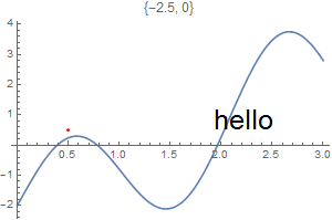
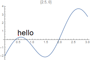
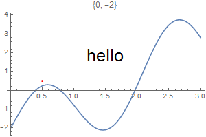
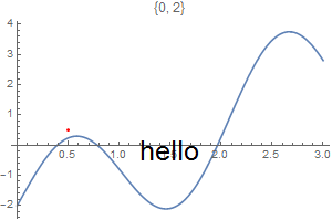
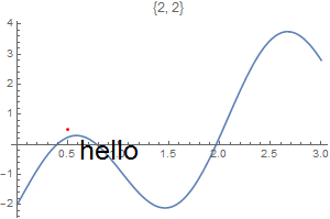
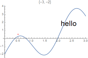
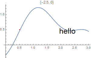
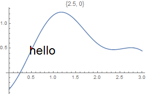
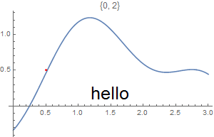
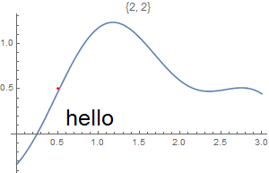
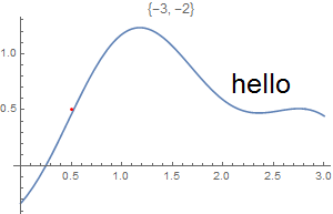
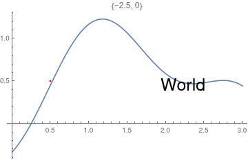
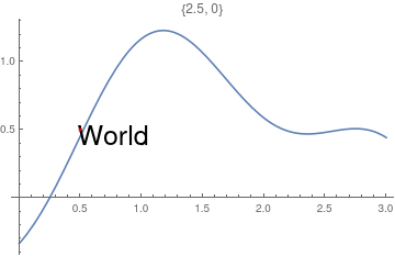
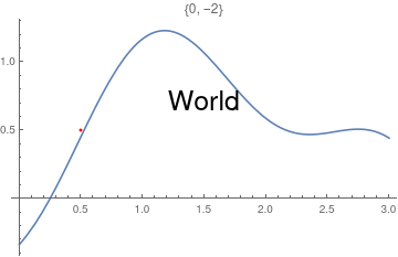
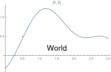
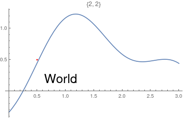
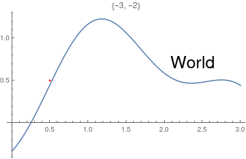
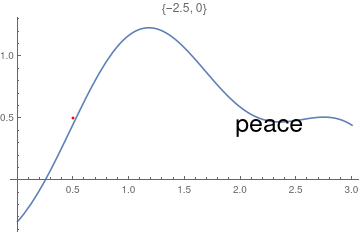
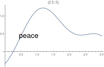
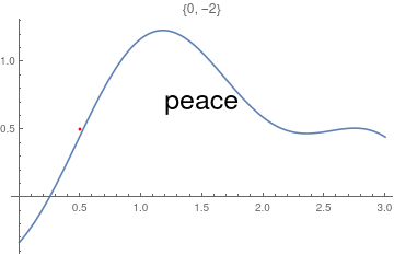
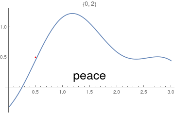
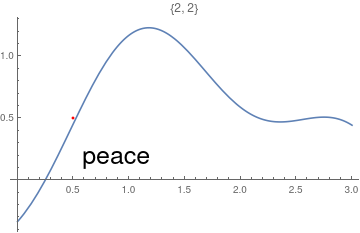
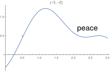
This chapter demonstrates Mathematica capability to generate graphs. We start with its basic command Plot and expose its ability to add text into figures. To place a text inside a figure, Mathematica has a special command Text[expr, coordinates, offset] that specifies an offset for the block of text relative to the coordinate given. Providing an offset { dx, dy } specifies that the point ( x, y ) should lie at relative coordinates { dx, dy } within the bounding rectangle that encloses the text. We demonstrate it with the following codes:

However, when we change dimensions of the graph, the text is displayed differently. The following table of graphs can be displayed using GraphicsGrid command. GraphicsGrid by default puts a narrow border around each of the plots in the array it gives. You can change the size of this border by setting the option Spacings -> { h, v} . The parameters h and v give the horizontal and vertical spacings to be used. The Spacings option uses the width and height of characters in the default font to scale the h and v parameters by default, but it is generally more useful in graphics to use Scaled coordinates. Scaled scales widths and heights so that a value of 1 represents the width and height of one element of the grid. How to add text to a graph, see
http://reference.wolfram.com/language/howto/AddTextToAGraphic.html.en
To add test outside the picture, see
http://reference.wolfram.com/language/howto/AddTextOutsideThePlotArea.html.en
The general reference is
http://reference.wolfram.com/language/howto/AddTextToAGraphic.html

 

There are someother options.

 

 

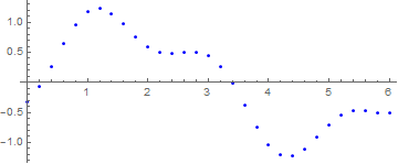
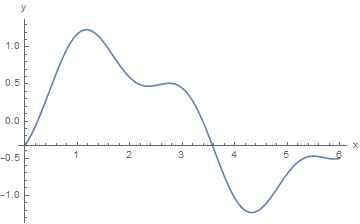
A graphic of a function can be made discrete:

We can shift the origin to another point, as the following example shows.

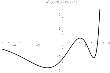
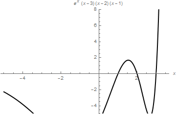
When you need to restrict the vertical range, use PlotRange command as the following example shows.