Preface
This tutorial was made solely for the purpose of education and it was designed for students taking Applied Math 0330. It is primarily for students who have very little experience or have never used Mathematica and programming before and would like to learn more of the basics for this computer algebra system. As a friendly reminder, don't forget to clear variables in use and/or the kernel. The Mathematica commands in this tutorial are all written in bold black font, while Mathematica output is in normal font.
Finally, you can copy and paste all commands into your Mathematica notebook, change the parameters, and run them because the tutorial is under the terms of the GNU General Public License (GPL). You, as the user, are free to use the scripts for your needs to learn the Mathematica program, and have the right to distribute this tutorial and refer to this tutorial as long as this tutorial is accredited appropriately. The tutorial accompanies the textbook Applied Differential Equations. The Primary Course by Vladimir Dobrushkin, CRC Press, 2015; http://www.crcpress.com/product/isbn/9781439851043
Return to computing page for the second course APMA0340
Return to Mathematica tutorial for the first course APMA0330
Return to Mathematica tutorial for the second course APMA0340
Return to the main page for the course APMA0330
Return to the main page for the course APMA0340
Return to Part II of the tutorial
Glossary
We need the following result that follows from the linearization procedure.
Theorem: Suppose y* is an equilibrium point (that is, \( f\left( y^{\ast} \right) =0 \) ) of the differential equation \( {\text d}y / {\text d}t = f\left( y \right) , \) where f is a continuously differentiable function. Then,
- if \( f\left( y^{\ast} \right) < 0 , \) then y* is a sink;
- if \( f\left( y^{\ast} \right) > 0, \) then y* is a source;
- if \( f\left( y^{\ast} \right) =0 , \) then we need additional information to determine the type of y*.
Bifurcation
Many of the equations that we have examined have a parameter, which means that we actually have a family of differential equations. For example, the logistic equation
A bifurcation diagram for a parameterized family of autonomous differential equations depending on a parameter k, \( {\text d}y /{\text d}t = f(y;k) , \) is a diagram in the ky-plane that summarizes the change in qualitative behavior of the equation as the parameter k is varied. The word bifurcate means “to divide into two parts or branches.” Hence, a bifurcation diagram shows us at what parameter values additional solutions emerge (or disappear). The bifurcation diagram is constructed by plotting the parameter value k against all corresponding equilibrium values \( y^{\ast} . \) Typically, k is plotted on the horizontal axis and critical points y* on the vertical axis. A "curve" of sinks is indicated by a solid line and a curve of sources is indicated by a dashed line. The method of constructing bifurcation diagrams should become evident as we study the following examples.
We need to make an observation that bifurcation occurs at the point \( \left( k_{0} , y^{\ast} \right) \) only when
- if y* is a sink with \( f\left( y^{\ast} \right) < 0 , \) then for all k sufficiently close to k0 the critical point y* remains a sink because the inequality \( f\left( y^{\ast} \right) < 0 \) holds in some neighborhood of the equilibrium point;
- if y* is a source with \( f\left( y^{\ast} \right) > 0, \) then for all k sufficiently close to k0 the critical point y* remains a source because the inequality \( f\left( y^{\ast} \right) > 0 \) holds in some neighborhood of the equilibrium point.
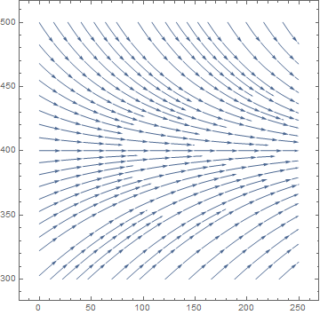
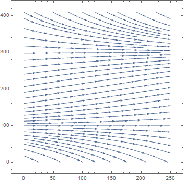
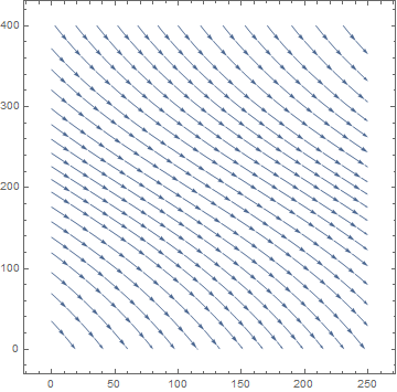
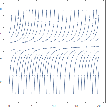
Example (Logistic Model with Harvesting). We model logistic growth in a trout pond with the equation
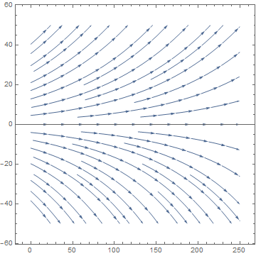
StreamPlot[{1, y*(1 - y/400)/100}, {x, 0, 250}, {y, -50, 50}, Frame -> True, Axes -> True]
 |
 |
To find a critical value of H, we solve the quadratic equation
b = Plot[1 + Sqrt[1 - H], {H, -1, 1}, PlotStyle -> {Thick, Blue}];
Show[a, b, PlotRange -> {{-1, 1}, {-0.5, 2.5}}]
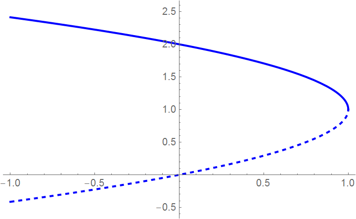
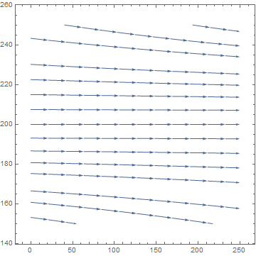
When H exceeds 1, all trajectories decline and the population dies out independently on the initial conditions.
Example: Let us consider the autonomous equation
For k = 0, the differential equation becomes
Example: Let us find the bifurcation values of the one-parameter family
I. Saddle-node bifurcation
A saddle-node bifurcation is a local bifurcation in which two (or more) critical points (or equilibria) of a differential equation (or a dynamic system) collide and annihilate each other. Saddle-node bifurcations may be associated with hysteresis and catastrophes.
Consider the slope function \( f(x, \alpha ) , \) where α is a control parameter. In this example, we use α instead of k because we need clearly distinguish a parameter (Greek letter α) from the variable (Latin letter y); we will return to k after rescaling. Then the solutions of the autonomous differential equation \( x' = f(x, \alpha ) \) and critical points (if any) will also depend on this parameter α. If we demand \( f(x, \alpha ) =0 \) and \( \partial_x f(x, \alpha ) =0, \) we get two equations in two unknowns, and in general there will be a zero-dimensional solution set consisting of points \( \left( x_c , \alpha_c \right) . \) Let’s expand \( f(x, \alpha ) \) in the vicinity of such a point \( \left( x_c , \alpha_c \right) : \)
b = Graphics[{Blue, Thick, Arrow[{{Sqrt[2] - 0.05, 0}, {-0, 0}}], Arrow[{{0, 0}, {-Sqrt[2] + 0.05, 0}}]}]
c = Graphics[Line[{{0, -2.02}, {0, 4}}]]
t1 = Graphics[Text[Style["u", FontSize -> 14, Black], {2.8, -0.3}]]
t2 = Graphics[Text[Style["f", FontSize -> 14, Black], {0.2, 2.9}]]
t3 = Graphics[Text[Style["r<0", FontSize -> 14, Black], {0.0, -2.3}]]
b1 = Graphics[{Red, Thick, Arrow[{{Sqrt[2] + 0.1, 0}, {2, 0}}], Arrow[{{2, 0}, {3, 0}}]}]
b2 = Graphics[{Red, Thick, Arrow[{{-2, 0}, {-Sqrt[2] - 0.1, 0}}], Arrow[{{-3, 0}, {-2, 0}}]}]
st = Graphics[{PointSize[Large], Point[{Sqrt[2], 0}]}]
circle = Graphics[Circle[{-Sqrt[2], 0}, 0.05], AspectRatio -> 1]
Show[a, b, c, t1, t2, t3, b1, b2, circle, st, AspectRatio -> 1, PlotRange -> {{-3, 3}, {-2.1, 3}}]
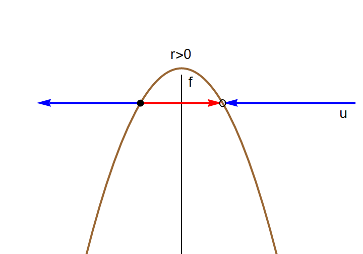
c = Graphics[Line[{{0, -0.02}, {0, 4}}]]
t1 = Graphics[Text[Style["u", FontSize -> 14, Black], {2.8, -0.3}]]
t2 = Graphics[Text[Style["f", FontSize -> 14, Black], {0.2, 2.9}]]
t3 = Graphics[Text[Style["r=0", FontSize -> 14, Black], {0.0, -0.3}]]
b1 = Graphics[{Red, Thick, Arrow[{{0.01, 0}, {2, 0}}], Arrow[{{2, 0}, {3, 0}}]}]
b2 = Graphics[{Red, Thick, Arrow[{{-2, 0}, {-0.1, 0}}], Arrow[{{-3, 0}, {-2, 0}}]}]
circle = Graphics[Circle[{0, 0}, 0.05], AspectRatio -> 1]
Show[a, c, t1, t2, t3, b1, b2, circle, AspectRatio -> 1, PlotRange -> {{-3, 3}, {-2.1, 3}}]
c = Graphics[Line[{{0, -0.02}, {0, 4}}]]
t1 = Graphics[Text[Style["u", FontSize -> 14, Black], {2.8, -0.3}]]
t2 = Graphics[Text[Style["f", FontSize -> 14, Black], {0.2, 2.9}]]
t3 = Graphics[Text[Style["r=0", FontSize -> 14, Black], {0.0, -0.3}]]
b1 = Graphics[{Red, Thick, Arrow[{{0.02, 0}, {2, 0}}], Arrow[{{2, 0}, {3, 0}}]}]
b2 = Graphics[{Red, Thick, Arrow[{{-2, 0}, {-0.02, 0}}], Arrow[{{-3, 0}, {-2, 0}}]}]
Show[a, c, t1, t2, t3, b1, b2, AspectRatio -> 1, PlotRange -> {{-3, 3}, {-2.1, 3}}]
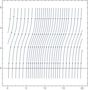
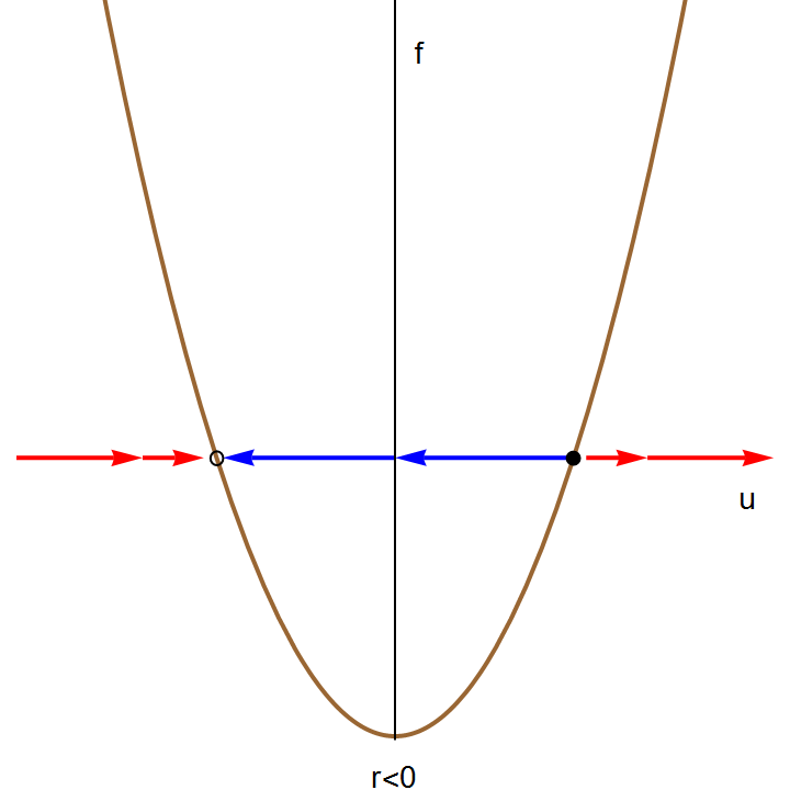
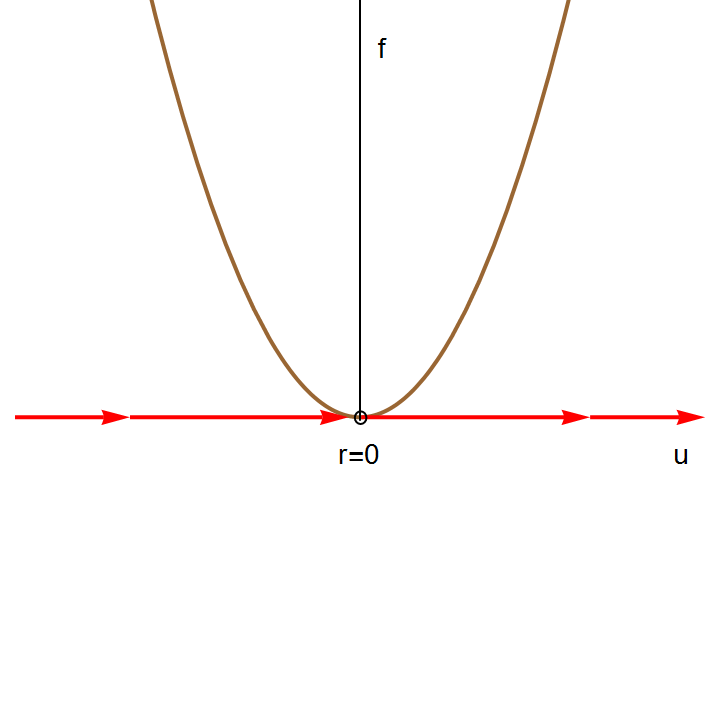
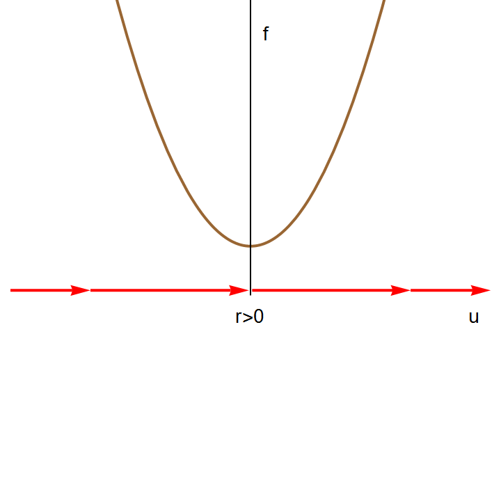
The right-hand side of this differential equation is the function \( f(u;k) = k+ u^2 \) that depends continuously on the parameter k. If we graph this function as a function of u for different values of k to determine equilibria, we see that for k < 0, there are two equilibria, which disappear when k becomes positive.
 |
 |
 |
 |
 |
 |
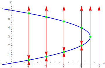
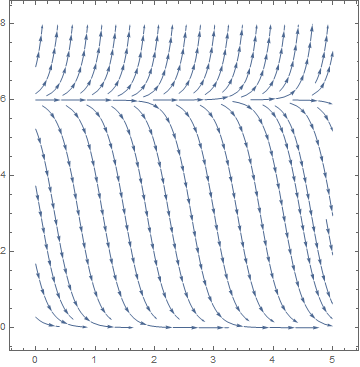
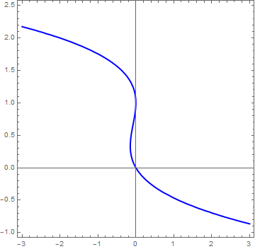
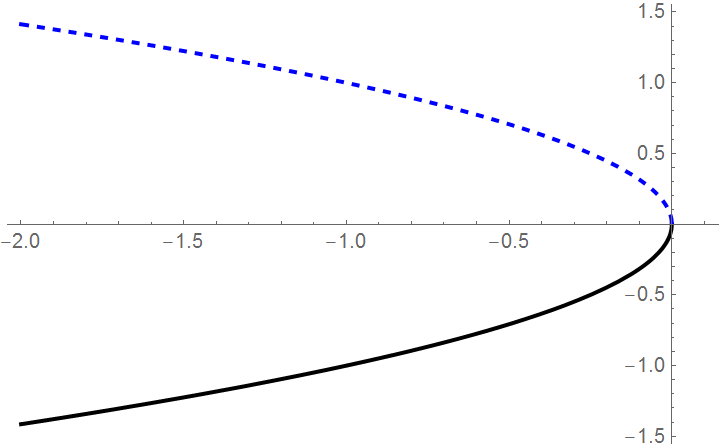
We can also graph the equilibria as functions of k. This figure is another example of a bifurcation diagram. For k < 0, there are two fixed points -- one stable (\( u^{\ast} = - \sqrt{-k} \) ) and one unstable (\( u^{\ast} = + \sqrt{-k} \) ). At k = 0, these two nodes coalesce and annihilate each other. (The point u* = 0 is half-stable precisely at k = 0.) For k > 0, there are no longer any fixed points in the vicinity of u = 0. In the left panel of Figure, we show the flow in the extended (k,u) plane. The unstable and stable nodes annihilate at k = 0.
b = Plot[Sqrt[-x], {x, -2, 0}, PlotStyle -> {Dashed, Thick, Blue}]
Show[a, b, PlotRange -> {{-2, 0.1}, {-1.4, 1.4}}]
It is possible to calculate the time it takes a solution starting at \( -\infty \) at τ=0 to reach \( \infty \) at τ = T. We can find T by solving the differential equation \( \dot{u} = k + u^2 \) with the conditions \( u(0) = -\infty \) and \( u(T) = \infty . \) We separate variables and compute the following definite integrals:
II. Transcritical bifurcation
A transcritical bifurcation is a particular kind of local bifurcation when stability of critical points changes as the parameter is varied. In other words, the unstable fixed point becomes stable and vice versa. A critical point under a transcritical bifurcation is never destroyed, it just interchanges its stability with another critical point.
Another situation which arises frequently is the transcritical bifurcation. Consider the equation \( \dot{y} = f(y) \) in the vicinity of a fixed point y*.
Example. Consider a crude model of a laser threshold. Let n be the number of photons in the laser cavity, and N the number of excited atoms in the cavity. The dynamics of the laser are approximated by the equations
III. Pitchfork bifurcation
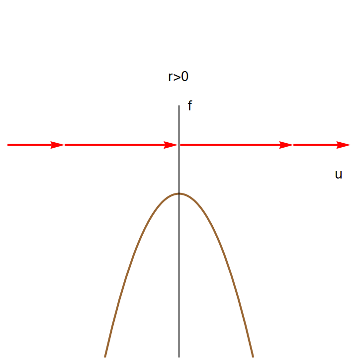
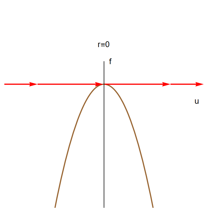
The pitchfork bifurcation is commonly encountered in systems in which there is an overall parity symmetry (\( u\,\mapsto -u . \) ). There are two classes of pitchfork: supercritical and subcritical. The normal form or generic model of the supercritical bifurcation is
If we send \( u\,\mapsto -u , \quad k\,\mapsto -k , \quad \mbox{and} \quad t\,\mapsto -t , \) we obtain the subcritical pitchfork, depicted in Figure. The normal form of the subcritical pitchfork bifurcation is
IV. Imperfect bifurcation
The imperfect bifurcation occurs when a symmetry-breaking term is added to the pitchfork. The normal form contains two control parameters:
This equation arises from a crude model of magnetization dynamics. Let M be the magnetization of a sample, and f(M) be the free energy. Assuming M is small, we can expand f(M) as
Fixed points satisfy the equation
V. Landau Theory of Phase Transitions
VI. Single Neuron Equation
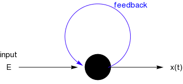
Consider a single neuron (nerve cell) that is receiving external input from surrounding cells in the brain, plus feedback from its own output,
Arrow[BSplineCurve[
Table[{0.5*Cos[x], 0.5*Sin[x] + 0.47}, {x, -Pi/3 - 0.2, Pi*4/3 + 0.2, Pi/20}]]]}]
disk = Graphics[Disk[{0, 0}, 0.2]]
arrow2 = Graphics[Arrow[{{0.2, 0}, {1, 0}}]]
arrow3 = Graphics[Arrow[{{-1.2, 0}, {-0.3, 0}}]]
text1 = Graphics[ Text[Style["feedback", FontSize -> 14, Blue], {0.5, 0.95}]]
text2 = Graphics[Text[Style["x(t)", FontSize -> 14, Black], {1.2, 0}]]
text3 = Graphics[Text[Style["E", FontSize -> 14, Black], {-1.35, 0}]]
text4 = Graphics[ Text[Style["input", FontSize -> 14, Black], {-1.35, 0.2}]]
Show[disk, arrow, arrow2, arrow3, text1, text2, text3, text4]
Let x(t) denote the level of activity of the neuron at time t, normalized to be between 0 (low activity) and 1 (high activity). A simple model representing the change of activity level for such a cell is given by the differential equation
The differential equation for x(t) becomes autonomous:
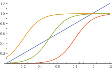
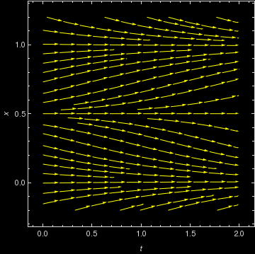
The equilibrium solutions of this slope functions are constant values of x, where \( x = S(x+E-\theta ) . \) The figure above shows graphs of y = x and the response function \( y = S(x+E-\theta ) \) for values θ = 0.4, 0.7, and 1.0 with a = 10 and E=0.2. It is seen that for small θ there will be one equilibrium solution near x = 1 and for large θ there will be one stationary solution near x = 0. This seems reasonable because a high threshold means it takes a lot of input to produce very much activity. For θ in a middle range, however, there can be three equilibrium solutions. WE want to determine the two bifurcation values of θ at which the number of stationary solutions changes from 1 to 3 and from 3 to 1. First, we plot direction field:
StreamPlot[{1, neuron[x, 10, 0.2, 0.7] - x}, {t, 0, 2}, {x, -0.2, 1.2},
StreamStyle -> Yellow, FrameStyle -> LightGray, Background -> Black, FrameLabel -> {t, x}]
- Abelson, H., The bifurcation interpreter: a step towards the automatic analysis of dynamic systems, Computers & Mathematics with Applications, 1990, Vol. 20, Issue 8, pp. 13--35.
Return to Mathematica page
Return to the main page (APMA0330)
Return to the Part 1 (Plotting)
Return to the Part 2 (First Order ODEs)
Return to the Part 3 (Numerical Methods)
Return to the Part 4 (Second and Higher Order ODEs)
Return to the Part 5 (Series and Recurrences)
Return to the Part 6 (Laplace Transform)
Return to the Part 7 (Boundary Value Problems)