Preface
The methods named after Carl Runge and Wilhelm Kutta (letter "u" in both last names is pronounced as in the word "rule") are designed to imitate the Taylor series method without requiring analytic differentiation of the original slope function. Recall the Taylor series in two variables:
Return to computing page for the second course APMA0340
Return to Mathematica tutorial for the first course APMA0330
Return to Mathematica tutorial for the second course APMA0340
Return to the main page for the course APMA0330
Return to the main page for the course APMA0340
Return to Part V of the course APMA0330
Glossary
Runge--Kutta Methods
 |
 |
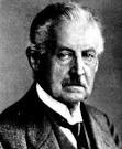
| Martin Kutta | Carl Runge |
In 1895 paper, the German mathematician Carl David Tolmé Runge (1856--1927) extended the approximation method of Euler to a more elaborate scheme which was capable of greater accuracy. He explored three main schemes, called now the midpoint method, the Heun method, and the trapezoid rule. Runge was very sporting, a fit and active man even as he grew older, and on his 70th birthday he entertained his grandchildren by doing handstands. Runge's son Wilhelm was an early developer of radar, and his daughter, Nerina (Nina), married the German American mathematician Richard Courant (1888-1972), who established one of America’s most prestigious institutes of applied mathematics and was co-author of the finite element method.
His immediate successors, the German mathematician Karl Heun (1859--1929) and Martin Wilhelm Kutta (1867--1944) layed down the foundations for a family of numerical methods known as the Runge--Kutta methods. In 1900, K. Heun analyzed some numerical methods and introduced amongst other methods the third order method used for the approximate solutions of ordinary differential equations. The paper by K.W. Kutta, which appeared in 1901, took the analysis of Runge--Kutta methods as far as order 5. He made a complete classification of order 4 methods and introduced the famous method, known now as the classical Runge--Kutta method. Besides being a co-developer of the Runge--Kutta method, Martin is also remembered for the Zhukovsky--Kutta aerofoil, the Kutta--Zhukovsky theorem, and the Kutta condition in aerodynamics.
The first phase in the history of Runge--Kutta methods ended in the work of the Finnish mathematician Evert Johannes Nyström (1895--1960), a former student of Lindelöf and a professor of applied mathematics at the Helsinki University of Technology. He took the analysis of fifth order methods to its completion but, more importantly, he extended the use of Runge--Kutta methods to
second order differential equation systems. These systems arise in dynamical problems and can often be solved more
efficiently when posed in their original form rather than as converted to an equivalent first order systems. Further work on Runge--Kutta methods was carried out by the Professor Anton Huta (born in 1915) of the University of Bratislava who took the analysis as far as order 6. The theory for a system comes out of the work of S. Gill, R.H. Merson, and John Charles Butcher (born in 1933) from the University of Auckland. A history of development of Runge--Kutta methods can be found in
Butcher, J.C., A history of Runge--Kutta methods, Applied Numerical Mathematics, 20 (1996) 247--260
Both previously discussed rules (improved Euler and modified Euler) are particular cases of a family of implicit and explicit iterative numerical methods known as the Runge--Kutta methods. The idea of Runge--Kutta methods is to take successive (weighted) Euler steps to approximate a Taylor series. In this way function evaluations (and not derivatives) are used.
For example, consider the one-step formulation of the midpoint method used to find a numerical solution to the initial value problem \( y' = f(x,y), \quad y(x_0 ) = y_0 . \)
Extending the above approach, repeated function evaluation can be used to obtain higher-order methods. Let us denote the Runge--Kutta approximation to the solution of the initial value problem \( y' = f(x,y) , \quad y(x_0 ) = y_0 \) at mesh point \( x_{n+1} = x_n +h \) by yn+1. Then
\]
Explicit Runge--Kutta methods are a special case where the matrix A is strictly lower triangular:
\]
Example: The Butcher table for the explicit midpoint method is given by:
The Euler’s method is sometimes called the first order Runge--Kutta Method, and the Heun’s method the second order one. In following sections, we consider a family of Runge--Kutta methods.
Explicit Runge--Kutta methods are generally unsuitable for the solution of stiff equations because their region of absolute stability is small. The instability of explicit Runge--Kutta methods motivates the development of implicit methods. An implicit Runge--Kutta method has the form
Example: Let us take a
Example: The simplest example of an implicit Runge--Kutta method is the backward Euler method:
V. Method Comparison
Sometimes you may be interested to find out what methods are being used in NDSolve.
Here you can see the coefficients of the default 2(1) embedded pair.
{{{1}, {1/2, 1/2}}, {1/2, 1/2, 0}, {1, 1}, {-(1/2), 2/3, -(1/6)}}
You also may want to compare some of the different methods to see how
they perform for a specific problem.
Implicit Runge--Kutta methods have a number of desirable properties.
The Gauss--Legendre methods, for example, are self-adjoint, meaning
that they provide the same solution when integrating forward or
backward in time.
http://reference.wolfram.com/language/tutorial/NDSolveImplicitRungeKutta.html
A generic framework for implicit Runge--Kutta methods has been implemented. The focus so far is on methods with interesting geometric properties and currently covers the following schemes:
"ImplicitRungeKuttaGaussCoefficients"
"ImplicitRungeKuttaLobattoIIIACoefficients"
"ImplicitRungeKuttaLobattoIIIBCoefficients"
"ImplicitRungeKuttaLobattoIIICCoefficients"
"ImplicitRungeKuttaRadauIACoefficients"
"ImplicitRungeKuttaRadauIIACoefficients"
The derivation of the method coefficients can be carried out to arbitrary order and arbitrary precision.
- explicit Runge--Kutta
- Butcher, J.C., A history of Runge--Kutta methods, Applied Numerical Mathematics, 20 (1996) 247--260
Return to Mathematica page
Return to the main page (APMA0330)
Return to the Part 1 (Plotting)
Return to the Part 2 (First Order ODEs)
Return to the Part 3 (Numerical Methods)
Return to the Part 4 (Second and Higher Order ODEs)
Return to the Part 5 (Series and Recurrences)
Return to the Part 6 (Laplace Transform)
Return to the Part 7 (Boundary Value Problems)