Return to computing page for the second course APMA0340
Return to Mathematica tutorial for the first course APMA0330
Return to Mathematica tutorial for the second course APMA0340
Return to the main page for the course APMA0330
Return to the main page for the course APMA0340
Return to Part V of the course APMA0330
Glossary
Discrete logistic recurrence
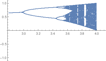
The logistic map is a polynomial mapping (equivalently, recurrence relation) of degree 2) that is describd by the recurrence:
t1 = Table[{r, Nest[f[r], .5, n]}, {r, 2.8, 4.1, 1.2/249}, {n, 101, 300}];
toshow = Flatten[t1, 1];
ListPlot[toshow, PlotRange -> {{3.7, 4}, {0; 1}}, PlotStyle -> PointSize[0.004]]
 |
 |
| Output of discrete logistic recurrence | Mandelbrot set |
|
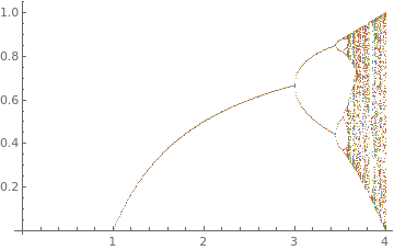
Discrete logistic recurrence:
ListPlot[Table[
Thread[{r, Nest[r # (1 - #) &, Range[0, 1, 0.01], 1000]}], {r, 0, 4,
0.01}]]
|
|
| Solutions of discrete logistic recurrence. | Mathematica code |
Example: Using real data and simply perform the least squares best fit of a quadratic function (without the constant term) through this data, we obtain the logistic grow model:
Hénon map

The map was introduced by Michel Hénon (1931--2013) as a simplified model of the Poincaré section of the Lorenz model. For the classical map, an initial point of the plane will either approach a set of points known as the Hénon strange attractor, or diverge to infinity. The Hénon attractor is a fractal, smooth in one direction and a Cantor set in another. As an example, consider the Standard Map:
Here b is the stochasticty parameter. For b = 0, the system corresponds for example to the ideal pendulum, exhibiting a completly regular motion. For b > 0, the pendulum is disturbed by a periodic driving force. This has the dramatic effect of producing stochastic orbits for certain initial conditions (i.e. points in phase space). The standard treatment of physics is to deal with the perturbation by expanding the driving force using a Taylor series and to keep only the linear part, with the understanding that higher order contributions are sufficiently small to be neglected. However, this treatment completely misses the qualitative aspects of the driven pendulum. With increasing b increasingly large fractions of phase space become chaotic. Chaotic orbits extend over a two-dimensional area in the above mapping plane. In addition, there are periodic orbits, indicated by a finite number of points on the mapping plane, and quasi-periodic orbits, which produce one or more closed lines (loops) in the mapping plane. Note that for conservative mappings, regular and chaotic phase space regions are arranged on many scales in a self-similar fashion, giving a strong indication that this structure is fractal.
- Chirikov, B. V. "A Universal Instability of Many-Dimensional Oscillator Systems." Phys. Rep. 52, 264-379, 1979.
- Cvitanović, P., Gunaratne, G., Procaccia, I., (1988). "Topological and metric properties of Hénon-type strange attractors". Physical Review A. 38 (3): 1503–1520. doi:10.1103/PhysRevA.38.1503.
- M. Hénon (1976). "A two-dimensional mapping with a strange attractor". Communications in Mathematical Physics. 50 (1): 69–77. doi:10.1007/BF01608556.
- Michel Hénon and Yves Pomeau (1976). "Two strange attractors with a simple structure,". Turbulence and Navier Stokes Equations. Springer: 29–68
- Luhn, A. Another interactive iteration of the Hénon Map.
- MacKay, R. S. and Percival, I. C. "Converse KAM: Theory and Practice." Comm. Math. Phys. 98, 469-512, 1985.
Return to Mathematica page
Return to the main page (APMA0330)
Return to the Part 1 (Plotting)
Return to the Part 2 (First Order ODEs)
Return to the Part 3 (Numerical Methods)
Return to the Part 4 (Second and Higher Order ODEs)
Return to the Part 5 (Series and Recurrences)
Return to the Part 6 (Laplace Transform)
Return to the Part 7 (Boundary Value Problems)