Return to computing page for the second course APMA0340
Return to Mathematica tutorial for the second course APMA0340
Return to Mathematica tutorial for the first course APMA0330
Return to the main page for the second course APMA0340
Return to the main page for the first course APMA0330
Return to Part III of the course APMA0330
Glossary
Runge--Kutta of order 2
The second order Runge--Kutta method (denoted RK2) simulates the accuracy of the Tylor series method of order 2. Although this method is not as good as the RK4 method, its derivation illustrates all steps and the principles involved. We consider the initial value problem \( y' = f(x,y) , \quad y(x_0 ) = y_0 \) that is assumed to have a unique solution. Using a uniform grid of points \( x_n = x_0 + n\, h , \) with fixed step size h, we write down the Taylor series formula for y(x+h):
The derivatives y' and y'' must be extressed in terms of f(x,y) and its partial derivatives according to the given differential equation \( y' = f(x,y) . \) So we have
Since there are only three equations in four unknowns, the system is underdetermined and we are permitted to choose one of the coefficients as we wish. There are several special choices that have been studied in the literature, and we mention some of them.
If we choose b1 = 1/2, this yields b2 = 1/2, c2 = 1, and a2,1 = 1. So we get Heun's method:
\begin{equation} \label{EqHeun} \begin{split} k_1 &= f\left( x_n , y_n \right) , \\ k_2 &= f\left( x_n , y_n + h\,k_1 \right) , \\ y_{n+1} &= y_n + \frac{h}{2} \left( k_1 + k_2 \right) , \qquad n=0,1,2,\ldots . \end{split} \end{equation}If we choose b1 = 0, this yields b2 = 1, c2 = 1/2, and a2,1 = 1/2. So we get the modified Euler method (also known as the explicit midpoint method):
\begin{equation} \label{EqmEuler} \begin{split} k_1 &= f\left( x_n , y_n \right) , \\ y_{n+1} &= y_n + h\, f\left( x_n + \frac{h}{2} , y_n + \frac{h}{2}\,k_1 \right) , \qquad n=0,1,2,\ldots . \end{split} \end{equation}Example:
The Butcher table for the explicit midpoint method is given by:
oneRK2[args_] :=
Module[{f, x0, y0, t0, k1, k2, h, x1, y1, t1, k12, k22},
{f, y0, t0, k1, k2, h} = args;
y1 = y0 + ((k1 + k2)/2.0);
t1 = t0 + h;
k12 = h*f[y0, t0];
k22 = h*f[y0 + k1, t0 + h];
{f, y1, t1, k12, k22, h} ];
- list
- line
- plot
- table
Module[{list, f, y0, t0, k1, k2, h, xy},
list = {};
{f, y0, t0, k1, k2, h} = args;
NestList[(AppendTo[list, {#, oneHeun[#]}]; oneHeun[#]) &, {f, y0, t0, k1, k2, h}, n];
(* this command executes the loop *)
xy = Table[{list[[i]][[1]][[3]], list[[i]][[1]][[2]]}, {i, 1, Length@list}];
<|
"list" -> list,
"poly line" -> xy,
"plot" -> ListLinePlot[xy, PlotRange -> All, AxesLabel -> syms, PlotStyle ->Thick],
"table" -> (Dataset@Table[ tmp = Drop[list[[i]][[1]], 1];
<|
syms[[1]] -> tmp[[2]], syms[[2]] -> tmp[[1]],
ToString[Subscript["k", 1], TraditionalForm] -> tmp[[3]],
"Subscript[k,2]" -> tmp[[4]]
ToString[Subscript["k", 2], TraditionalForm] -> tmp[[4]]
"Subscript[k,2]" -> tmp[[4]]
|>,
{i, 1, Length@list}])
|>
];
Example: We consider the initial value proble with oscillating slope function:
I. Second Order Optimal Runge-Kutta Approximation
Ralston's method is a second-order method with two stages and a minimum local error bound. Its Mathematica realization is presented below when the step size is denoted by h: \begin{equation} \label{E35.opt} y_{n+1} =y_n + \frac{h}{4}\,f(x_n , y_n ) + \frac{3h}{4} \,f\left( x_n + \frac{2h}{3} , y_n + \frac{2h}{3} \,f(x_n , y_n ) \right) , \quad n=0,1,2,\ldots . \end{equation} Its Butcher tableau is
Block[{xold = x0, yold = y0, sollist = {{x0, y0}}, x, y, n, steps,xnew, ynew,xthird,fn,k1},
steps = Round[(xn - x0)/h];
Do[xnew = xold + h;
xthird = xold + 2*h/3;
fn = f [x -> xold, yold];
k1 = f[xthird, yold + fn*2*h/3];
ynew = yold + h*fn/4 + 3*h*k1/4;
sollist = Append[sollist, {xnew, ynew}];
xold = xnew;
yold = ynew, {steps}];
Return[sollist[[steps + 1]]]]
RK2op[f, {1, 2}, 1, 0.1]
The same algorithm when the number of steps is specified:
Block[{xold = x0, yold = y0, sollist = {{x0, y0}}, x, y, n, h,
xthird, fn, ynew, xnew, k1}, h = N[(xn - x0)/steps];
Do[xnew = xold + h;
xthird = xold + 2*h/3;
fn = f[xold, yold];
k1 = f[xthird, yold + fn*2*h/3];
ynew = yold + h*fn/4 + 3*h*k1/4;
sollist = Append[sollist, {xnew, ynew}];
xold = xnew;
yold = ynew, {steps}];
Return[sollist]]
RK2ops[f, {1, 2}, 1, 10]
2.07271}, {1.5, 2.44234}, {1.6, 2.86129}, {1.7, 3.33472}, {1.8,
3.86837}, {1.9, 4.46855}, {2., 5.14224}}
If only one final value is needed, then Return command should be replaced with
II. Implicit Runge-Kutta of order 2
First we present code when the step size (h) is given:
Block[{xold = x0, yold = y0, sollist = {{x0, y0}}, steps},
steps = Round[(xn - x0)/h];
Do[xnew = xold + h;
fold = f /. {x -> xold, y -> yold};
sol = FindRoot[{f1 ==
1/(3*(xold + (Sqrt[3] - 1)/(2*Sqrt[3])*h) -
2*(yold + h/4*f1 + (Sqrt[3] - 2)/(4*Sqrt[3])*h*f2) + 1),
f2 == 1/(3*(xold + (Sqrt[3] + 1)/(2*Sqrt[3])*h) -
2*(yold + h/4*f2 + (Sqrt[3] + 2)/(4*Sqrt[3])*h*f1) +
1)}, {{f1, fold}, {f2, fold}}];
ynew = yold + (h/2)*(sol[[1, 2]] + sol[[2, 2]]);
sollist = Append[sollist, {xnew, ynew}];
xold = xnew;
yold = ynew, {steps}];
Return[sollist]]
Then the same algorithm when the number of steps is specified:
Block[{xold = x0, yold = y0, sollist = {{x0, y0}}, h},
h = N[(xn - x0)/steps];
Do[xnew = xold + h;
fold = f /. {x -> xold, y -> yold};
sol = FindRoot[{f1 ==
1/(3*(xold + (Sqrt[3] - 1)/(2*Sqrt[3])*h) -
2*(yold + h/4*f1 + (Sqrt[3] - 2)/(4*Sqrt[3])*h*f2) + 1),
f2 == 1/(3*(xold + (Sqrt[3] + 1)/(2*Sqrt[3])*h) -
2*(yold + h/4*f2 + (Sqrt[3] + 2)/(4*Sqrt[3])*h*f1) +
1)}, {{f1, fold}, {f2, fold}}];
ynew = yold + (h/2)*(sol[[1, 2]] + sol[[2, 2]]);
sollist = Append[sollist, {xnew, ynew}];
xold = xnew;
yold = ynew, {steps}];
Return[sollist]]
0.324916}, {0.5, 0.386028}, {0.6, 0.440961}, {0.7, 0.490565}, {0.8,
0.53558}, {0.9, 0.576638}, {1., 0.614275}}
Using Mathematica command NDSolve, we check the obtained value:
Block[{xold = x0, yold = y0, sollist = {{x0, y0}}, steps},
steps = Round[(xn - x0)/h];
Do[xnew = xold + h;
fold = f /. {x -> xold, y -> yold};
sol = FindRoot[{f1 ==
1/(3*(xold + (Sqrt[3] - 1)/(2*Sqrt[3])*h) -
2*(yold + h/4*f1 + (Sqrt[3] - 2)/(4*Sqrt[3])*h*f2) + 1),
f2 == 1/(3*(xold + (Sqrt[3] + 1)/(2*Sqrt[3])*h) -
2*(yold + h/4*f2 + (Sqrt[3] + 2)/(4*Sqrt[3])*h*f1) +
1)}, {{f1, fold}, {f2, fold}}];
ynew = yold + (h/2)*(sol[[1, 2]] + sol[[2, 2]]);
sollist = Append[sollist, {xnew, ynew}];
xold = xnew;
yold = ynew, {steps}];
Return[sollist]]
III. Ralston's method
The second order Ralston approximation can written as follows:
\begin{equation*} %\label{E35.ralston} y_{n+1} =y_n + \frac{h}{3}\,f(x_n , y_n ) + \frac{2h}{3} \,f\left( x_n + \frac{3h}{4} , y_n + \frac{3h}{4} \,f(x_n , y_n ) \right) , \quad n=0,1,2,\ldots . \end{equation*}Block[{xold = x0, yold = y0, sollist = {{x0, y0}}, x, y, n, h, xnew,
ynew, xthird, k1, fn}, h = N[(xn - x0)/steps];
Do[xnew = xold + h;
xthird = xold + 3*h/4;
fn = f[xold, yold];
k1 = f[xthird, yold + fn*3*h/4];
ynew = yold + h*fn/3 + 2*h*k1/3;
sollist = Append[sollist, {xnew, ynew}];
xold = xnew;
yold = ynew, {steps}];
Return[sollist[[steps + 1]]]]
Ralston2s[f, {1, 2}, 1, 10]
The same algorithm with fixed step size (which is denoted by h) is specified:
Block[{xold = x0, yold = y0, sollist = {{x0, y0}}, x, y, n, steps,
xnew, ynew, xthird, k1, fn}, steps = Round[(xn - x0)/h];
Do[xnew = xold + h;
xthird = xold + 3*h/4;
fn = f[xold, yold];
k1 = f[xthird, yold + fn*3*h/4];
ynew = yold + h*fn/3 + 2*h*k1/3;
sollist = Append[sollist, {xnew, ynew}];
xold = xnew;
yold = ynew, {steps}];
Return[sollist[[steps + 1]]]]
Ralston2[f, {1, 2}, 1, 0.1]
Actually, the Heun, midpoint, and Ralston methods could be united into one algorithm, based on a parameter, which we denote by a2. Select a value for a2 between 0 and 1 according to
- Heun Method: a2 = 0.5
- Midpoint Method: a2 = 1.0
- Ralston's Method: a2 = 2/3
Then Mathematica codes will need only one modification:
h=(xf-x0)/n;
Y=y0;
a1=1-a2;
p1=1/(2*a2);
q11=p1;
For[i=0,i<n,i++,
k1=f[x0+i*h,Y];
k2=f[x0+i*h+p1*h,Y+q11*k1*h];
Y=Y+(a1*k1+a2*k2)*h]; Y]
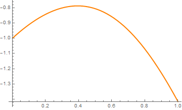
Example: Consider the initial value problem for the Riccati equation
x0=0.0; (* starting point *)
y0=-1.0; (* initial condition *)
xf=1.0; (* final value *)
n=128; (* maximum number of steps *)
a2=2/3 (* Ralston's Method *)
n = number of steps
x0 = boundary condition for x
y0 = boundary condition for y
xf = value of x at which y is desired
f = differential equation in the form dy/dx = f(x,y)
a2 = constant to identify the numerical method
First, we determine the true numerical value at the final point:
The following loop calculates the following quantiries:
AV = approximate value of the ODE solution usin
g second order RK method by calling the module RK2nd
Et = true error
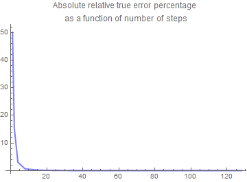
et = absolute relative true error percentage
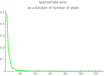
Ea = approximate error
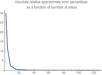
ea = absolute relative approximate error percentage
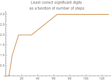
sig = least number of significant digits correct in approximation
Do[
Nn[i] = 2^i;
H[i] = (xf - x0)/Nn[i];
AV[i] = RK2nd[2^i, x0, y0, xf, f, a2];
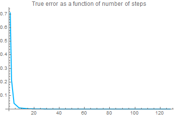
Et[i] = EV - AV[i];
et[i] = Abs[(Et[i]/EV)]*100.0;
If[i > 0,
Ea[i] = AV[i] - AV[i - 1];
ea[i] = Abs[Ea[i]/AV[i]]*100.0;
sig[i] = Floor[(2 - Log[10, ea[i]/0.5])];
If[sig[i] < 0, sig[i] = 0]; ] , {i, 0, nth}];
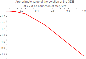
plot2 = ListPlot[data, Joined -> True,
PlotStyle -> {Thickness[0.006], RGBColor[1, 0, 0]}, PlotLabel ->
"Approximate value of the solution of the ODE\nat x = xf as a \ function of step size"]
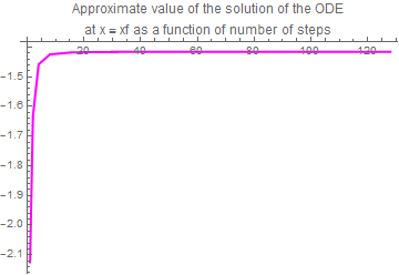
plot3 = ListPlot[data, Joined -> True,
PlotStyle -> {Thickness[0.006], RGBColor[1, 0, 1]}, PlotLabel ->
"Approximate value of the solution of the ODE\nat x = xf as a \ function of number of steps"]
plot4 = ListPlot[data,
AxesOrigin -> {0, 0}, Joined -> True,
PlotStyle -> {Thickness[0.006], RGBColor[0, 0.7, 1]},
PlotLabel -> "True error as a function of number of steps"]
plot5 = ListPlot[data,
AxesOrigin -> {0, 0}, Joined -> True,
PlotStyle -> {Thickness[0.006], RGBColor[0.5, 0.5, 1]}, PlotLabel ->
"Absolute relative true error percentage \nas a function of number \ of steps"]
plot6 = ListPlot[data, AxesOrigin -> {0, 0}, Joined -> True,
PlotStyle -> {Thickness[0.006], RGBColor[0, 1, 0]},
PlotLabel -> "Approximate error \nas a function of number of steps"]
plot7 = ListPlot[data, AxesOrigin -> {0, 0}, Joined -> True,
PlotStyle -> {Thickness[0.006], RGBColor[0, 0.3, 0.7]}, PlotLabel ->
"Absolute relative approximate error percentage \nas a function of \ number of steps"]
plot8 = ListPlot[data, AxesOrigin -> {0, 0}, Joined -> True,
PlotStyle -> {Thickness[0.006], RGBColor[0.80, 0.52, 0.25]}, PlotLabel ->
"Least correct significant digits \nas a function of number of \ steps"]
IV. Generic second-order method
Return to Mathematica page
Return to the main page (APMA0330)
Return to the Part 1 (Plotting)
Return to the Part 2 (First Order ODEs)
Return to the Part 3 (Numerical Methods)
Return to the Part 4 (Second and Higher Order ODEs)
Return to the Part 5 (Series and Recurrences)
Return to the Part 6 (Laplace Transform)
Return to the Part 7 (Boundary Value Problems)