Return to computing page for the first course APMA0330
Return to computing page for the second course APMA0340
Return to Mathematica tutorial for the first course APMA0330
Return to Mathematica tutorial for the second course APMA0340
Return to the main page for the course APMA0330
Return to the main page for the course APMA0340
where \( \texttt{D} = {\text d} / {\text d}x \) is the derivative operator (with respect to independent variable x), D0 = I is the identical operator, and coefficients 𝑎0(x), 𝑎1(x), … , 𝑎n(x) are continuous functions on some interval |𝑎, b|. Recall that we denote by |𝑎, b| any interval (open, closed or semi-open) with end points 𝑎 and b, assuming that 𝑎 < b. To every such linear differential operator corresponds either the homogeneous (not pronounce like milk) differential equation
where f(x) is a driving function or nonhomogeneous term (assumed to be continuous on the same interval). On an interval where the leading coefficient is not zero, 𝑎n ≠ 0, it can be factored out and on this interval we can always assume that 𝑎n = 1.
The second order linear differential equation has the form
the second order equation can be reduced to the normal form:
\[
v'' + \left( q - p^2 /4 -p' /2 \right) v = g
\]
that does not contain the the derivative of an unknown function v.
Linear differential equations form an important class of differential equations that appear both in physical models and as approximations for more complicated nonlinear equations. Out of them, the second order equations are of crucial importance in the theory of differential equations for two main reasons. First of all, the second order equations are often follows from basic physical law such as Newton's second law. Second, these equations serve as approximations in more complicated models. Further, a study of second order equations helps to understand the general theory of n-th order linear differential equations and provide illustrations for basic methods involved.
Example:
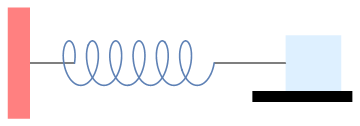
Suppose that we have a horizontal spring connected to a wall with a constant mass m attached. We assume that the total force F is made up of three forces:
Fs = force exerted by the spring;
Fr = a friction or resistive force acting on the mass;
Fe = any other external force (such as magnetism).
Let ℓ be the length of the spring with no mass attached. We introduce a coordinate system in which x = 0 is located a distance ℓ from the wall. Then x(t) is the distance of the mass from this position.
If x>0, then the spring is stretched. If x<0, the spring is compressed. If x = 0, then the spring is in a state of equilibrium. If we pull on the mass, then the mass will oscillate back and forth across the table.
We can construct a differential equation that models our oscillating mass. First, we must consider the restorative force on the spring. We will make the assumption that this force depends on the displacement of the spring, F(x). Using Taylor's Theorem from calculus, we can expand F to obtain
where \( F' (0) =-k \) and F(0) = 0. If the displacement is not too large, then xn will be small for \( n \ge 2, \) and we can ignore higher ordered terms. Thus, we can consider the restorative force on the spring to be proportional to displacement of the spring from its equilibrium length,
\[
F(x) \approx - k\,x .
\]
This equation is known as is Hooke's Law. We can test this law experimentally, and it is reasonably accurate if the displacement of the spring, x, is not too large.
By Newton's second law of motion, the force on the mass m must be
\[
F(x) = m\, \ddot{x} .
\]
Setting the two forces equal, we have a second order differential equation,
\[
m\, \ddot{x} = -k\, x \qquad\mbox{or} \qquad \ddot{x} + \omega^2 x =0 ,
\]
where \( \omega^2 = k/m , \) which depends on our oscillating mass. The spring-mass system is an example of a harmonic oscillator.
Now let us add a damping force to our system. For example, we might add a dashpot, a mechanical device that resists motion, to our system. Think of a dashpot as the small cylinder that keeps your screen door from slamming shut. The simplest assumption would be to take the damping force of the dashpot to be proportional to the velocity of the mass, \( \dot{x}(t) . \) Thus, we have will have an additional force, \( F(x) = -b\,\dot{x}(t) , \) acting on our mass, where b > 0. Our new equation for the spring-mass system is
\[
m\,\ddot{x} + b\,\dot{x} + k\, x =0 .
\]
■
Example:
A spring is an object that can be deformed by a force and then return to its original shape after the force is removed. Springs come in a huge variety of different forms, but what they all share is the elasticity. This term represents the reaction of a spring (or any other object) on axial load. When a force is placed on a material, the material stretches or compresses in response to the force. When the force is removed, the material returns to its original form.
When studying springs and elastic deformations, the 17ᵗʰ century British physicist Robert Hooke noticed that the stress vs strain curve for many materials has a linear region. Such proportionally of the extension of the spring to the applied force is known now as Hooke's law. Robert Hooke (1635--1703) was a scientist with wide-ranging interests. He published the book Micrographia in 1665 where he first formulated the law named after him.
Consider a mass m hanging at rest on the end of a vertical spring of original length \( \ell . \) The mass causes an elongation L of the spring in the downward direction, which we assume positive. In this static situation there are two forced acting at the point where the mass is attached to the spring. The gravitational force, or weight of the mass, acts downward and has magnitude mg, where g is the acceleration due to gravity. There is also a force, which we denote as F, due to the spring that acts upward. If we assume that the elongation L of the spring is small, the spring force is very nearly proportional to L: \( F = -k\,L , \) where k is called the spring constant. Since the mass is in equilibrium, the two forces balance each other, which means that
\[
mg - k\,L =0
\]
This mass m is pushed into the motion either by an external force or by initial displacement or by both. Let x(t), measured positive downward, denote the displacement of the mass from its equilibrium position at time t. Then x(t) is related to the forces acting on the mass according Newton's law of motion
\[
m\,\ddot{x} (t) = f(t) ,
\]
where \( \ddot{x} \) is the acceleration of the mass and f is the net force acting on the mass. Observe that there are now four separate forces to be considered:
The weight w = mg of the mass always acts downward.
The spring force Fs is assumed to be proportional to the total elongation L+x of the spring and always acts to restore the spring to its natural position. If L+x is positive, then the spring is extended, and the spring force is directed upward. In this case
\[
F_s = -k \left( L+x \right) .
\]
On the other hand, if L+x is negative, then the spring is compressed a distance |L+x|, and the spring force, which is now directed downward, is given by \( F_s = k\left\vert L+x \right\vert = -k \left( x+L \right) . \)
The damping or resistive force Fr always acts in the direction opposite to the direction of motion of the mass. This force may be caused by different sources: internal dissipation due to compression or extension of the spring, resistance from the air or other medium, friction between the mass and the guides that constrain its motion in one dimension, or a mechanical device that imparts a resistive force to the mass. We assume that the resulting resistive force is proportional to the speed, which is usually is referred to as viscous damping:
\[
F_r = -\gamma \,\dot{x} ,
\]
where γ is a positive constant of proportionality known as the damping constant.
Usually, a damping force is difficult to model---we discuss this issue in section devoted to pendulum motion. We benefit from this simple resistive force formula because the resulting differential equation becomes linear.
An applied external force F(t) could be either positive or negative depending in what direction it acts and at what time. Often the external force is periodic.
Taking into account all these forces, we obtain the following equation of motion:
Example:
Interestingly enough, the problem is as current today as it was in 1877.
A simple RLC circuit in series is shown below.
RLC circuit in series
Even the very simplest RLC circuits lead to integro-differential equations. For if a single-loop circuit contains resistance R, capacitance C, and inductance L with impressed voltage E(t), then Kirchhoff's second law yields
for linear second order differential operator L[x,D] = D² + p D + q I. It is assumed that the
coefficients p(x), q(x), and the driving term f(x) are continuous on an open interval (𝑎,b) that contains the point x0. Then there is exactly one solution y = ϕ(x) of this problem and the solution exists throughout the interval (𝑎,b).
This statement is valid also for arbitrary n-th order linear differential operator with continuous coefficients.
These functions p(x) and x(x) are continuous on the real axes ℝ except points
\[
\pm\pi , \pm 2\pi , \pm3\pi , \ldots ,
\]
but they are continuous at the origin. The initial point π/2 belongs to the interval π ∈ (-π, π), which is the longest interval in which all the coefficients are continuous.
If the initial condition will be specified at another point:
\[
y(4) = 1, \quad y' (4) = -1,
\]
then the longest interval of existence would be (π, 2π).
■
Theorem 2: If coefficients \( a_n (x), a_{n-1} (x), \ldots , a_0 (x) \)
are continuous functions on some interval |a,b| and \( a_n (x) \ne 0 , \) then the homogeneous
linear differential equation \( L \left[ x, \texttt{D} \right] y =0 , \) which can be written as
has n linearly independent solutions \( \left\{ y_1 (x), y_2 (x), \ldots , y_n (x) \right\} \)
that are continuous on the interval |a,b|. Then the general solution of the equation on the interval is
where \( C_1 , C_2 , \ldots , C_n \) are arbitrary constants. ⧫
The linear combination \( y_h (x) = C_1 \, y_1 (x) + C_{2} \, y_2 (x) + \cdots + a_{n-1} \, y_{n-1} (x) + a_n \, y_n (x) , \)
which is the general solution of the homogeneous equation \( L \left[ x, \texttt{D} \right] y = 0 \) is
sometimes called the complementary function for nonhomogeneous equation.
Theorem (Principle of Superposition for homogeneous equations):
If y1, y2, … , ym are solutions to some linear homogeneous differential equation L[x, D] y = 0, then their linear combination
is also a solution of the same homogeneous equation L[x, D] y = 0 for any values of constants c1, c2, … , cm.
It is convenient to use an operator notation L[x, D] y = f
for defining a differential equation. Recall that the zero power of the derivative operator is the identical operator: D0 = I.
The function f(x) in the right-hand side is called the nonhomogeneous term or driving term or forcing term.
Any function y = ϕ(x) that satisfies the above equation is called a particular solution of equation L[D] y = f. We usually identify a particular solution by subscript p: yp. The general solution (containing n arbitrary constants) of the homogeneous linear differential equation
L[D] y = 0 is denoted by yh.
Example:
Verify that \( y_p (x) = \frac{1}{32} \left( 8\,x^2 - 4\,x -7 \right) \) is a particular solution of \( y'' - 3\,y' + 4\,y = x^2 -2\,x . \)
Solution: Upon defining yp with Mathematica
yp[x_] = (8 x^2 - 4 x -7)/32
we compute and simplify \( y''_p - 3\,y'_p + 4\,y_p : \)
Simplify[yp''[x] -3 yp'[x] + 4 yp[x]]
(-2 + x) x
and see that the result is identically equal to the driven term.
■
Theorem 4:
Let yp be any particular solution of the nonhomogeneous linear n-th
order differential equation
on an interval |𝑎,b|, and let \( \left\{ y_1 (x), y_2 (x), \ldots , y_n (x) \right\} \)
be a fundamental set of solutions of the associated homogeneous differential equation
\( L \left[ x, \texttt{D} \right] y =0 \) on |𝑎,b|. Then the general solution
of the nonhomogeneous equation \( L \left[ x, \texttt{D} \right] y = f(x) \) on the interval is
where \( C_1 , C_2 , \ldots , C_n \) are arbitrary constants.
As we see from the previous Theorem, the general solution of a nonhomogeneous linear equation consists of the sum of two functions:
\[
y (x) = y_p (x) + y_h (x) ,
\]
In other words, to solve a
nonhomogeneous linear differential equation \( L \left[ x, \texttt{D} \right] y = f(x) \)
we first solve the associated homogeneous equation \( L \left[ x, \texttt{D} \right] y = 0 \)
and then find any particular solution of the nonhomogeneous equation.
Theorem (Principle of Superposition for nonhomogeneous equations):
If y1 and y2 are solutions to some linear driven differential equation L[x, D] y = f, then their linear combination
\[
y(x) = c_1 y_1 (x) + c_2 y_2 (x)
\]
is a solution of the following nonhomogeneous equation L[x, D] y = (c1 + c1) f for any values of constants c1, c2. In particular, if c1 + c2 = 0, their linear combination is a solution of the homogeneous equation L[x, D] y = 0.
If all coefficients of the linear differential operator \( L \left[ \texttt{D} \right] \)
are constants, then the general solution of the corresponding homogeneous equation \( L \left[ x, \texttt{D} \right] y = 0 \)
exist for all x on real axis. In this case, it is possible to find the fundamental set of solutions explicitly.
Following Leonhard Euler, we seek solutions to the homogeneous linear constant coefficient equation
as exponential function \( y (x) = e^{\lambda\,x} , \) for some parameter λ. Substituting
the exponential function into the homogeneous equation, we get
The polynomial of degree n, denoted by \( L(\lambda ) , \) is called the
characteristic polynomial corresponding to the linear constant coefficient differential operator
\( L \left[ \texttt{D} \right] = a_n \texttt{D}^n + \cdots + a_1 \texttt{D} + a_0 . \)
If the characteristic equation \( L(\lambda ) =0 \) has n distinct roots (real or complex),
we get n linearly independent exponential solutions that constitute the fundamental set of solutions for the
given homogeneous linear constant coefficient differential equation.
Example:
We consider the second order linear differential operator:
The corresponding characteristic polynomial \( L(\lambda ) = \lambda^2 - \lambda -6 = (\lambda +2)(\lambda -3) \)
has two distinct real roots \( \lambda =-2 \) and \( \lambda = 3 . \)
Then the functions \( y_1 (x) = e^{-2x} \) and \( y_2 (x) = e^{3x} \)
form a fundamental set of solutions, and the general solution to \( L \left[ x, \texttt{D} \right] y = 0 \) is
\[
y(x) = C_1 e^{-2x} + C_2 e^{3x} ,
\]
where C1 and C1 are arbitrary constants.
roots = Solve[s^2 - s - 6 == 0, s]
first = s /. roots[[1]]
second = s /. roots[[2]]
root = {first, second}
Soln = Map[Exp[# x] &, root]
{E^(-2 x), E^(3 x)}
AllSoln[x_]=Soln.{c1,c2}
Out[17]= c1 E^(-2 x) + c2 E^(3 x)
Simplify[L[x, AllSoln] == 0] (* check the answer *)
Out[18]= True
DSolve[y''[x] - y'[x] - 6 y[x] == 0, y[x], x]
■
Example:
A particular interest is a second order differential equation. Let us consider the equation of motion for
undriven damped harmonic oscillator (coefficients μ and ω0 > 0 are assumed constants)
\[
\ddot{y} + 2\mu\,\dot{y} + \omega_0^2 y =0 ,
\]
subject to the initial conditions
\[
y(0) = y_0 , \qquad \dot{y}(0) = v_0 .
\]
Assuming that the roots of the characteristic equation \( \lambda^2 + 2\mu\,\lambda + \omega_0^2 =0 \)
are distinct,
the differential equation has two linearly independent solutions
\( y_{1,2} = e^{\lambda_{1,2} t} . \)
Then the solution (which is unique) of the given initial value problem can be expressed as
The corresponding characteristic polynomial \( L(\lambda ) = \lambda^3 -2\,\lambda^2 - 5\,\lambda +6 = (\lambda -1)(\lambda +2)(\lambda -3) \)
has three distinct real roots \( \lambda =1, \) \( \lambda =-2 , \) and \( \lambda = 3 . \)
Then the functions \( y_1 (x) = e^{x} , \quad y_1 (x) = e^{-2x} , \) and \( y_3 (x) = e^{3x} \)
form a fundamental set of solutions, and the general solution to \( L \left[ x, \texttt{D} \right] y = 0 \) is
Return to Mathematica page
Return to the main page (APMA0330)
Return to the Part 1 (Plotting)
Return to the Part 2 (First Order ODEs)
Return to the Part 3 (Numerical Methods)
Return to the Part 4 (Second and Higher Order ODEs)
Return to the Part 5 (Series and Recurrences)
Return to the Part 6 (Laplace Transform)
Return to the Part 7 (Boundary Value Problems)