Preface
This chapter is supposed to help you with developing very important skills---plotting. Fortunately, Mathematica has a tremendous arsenal of tools to accomplish almost any plotting task. This chapter remembers that the presented material is for beginners and more advanced codes could be found elsewhere, in particular, in the second part of this tutorial.
Return to computing page for the second course APMA0340
Return to computing page for the fourth course APMA0360
Return to Mathematica tutorial for the first course APMA0330
Return to Mathematica tutorial for the second course APMA0340
Return to Mathematica tutorial for the fourth course APMA0360
Return to the main page for the course APMA0330
Return to the main page for the course APMA0340
Return to the main page for the course APMA0360
Glossary
Plotting
One of the best characteristics of Mathematica is its plotting ability. It is very easy to visualize diversity of outputs generated by Mathematica. This computer algebra system has a variety of two-dimensional plotting commands:
- Plot
- DiscretePlot
- ListPlot
- ListLinePlot
- NumberLinePlot
- LogPlot
- ListLogPlot
- LogLinearPlot
- LogLogPlot
- ParametricPlot
- PolarPlot
- ListPolarPlot
- PieChart
- BarChart
- SectorChart
- ContourPlot
- RegionPlot
- Graph
- GraphPlot
- UndirectedEdge
- DirectedEdge
- TreePlot
- AdjacencyGraph
- IncidenceGraph
- LayeredGraphPlot
- PathGraph
- Graphics
- GraphicsGrid
- GraphicsRow
- GraphicsColumn
- Grid
- Inset
- RegionUnion

In addition, Mark A. Caprio from the University of Notre Dame prepared a package SciDraw for preparing publication-quality scientific figures with Mathematica. SciDraw provides both a framework for structuring figures and tools for generating their content. SciDraw helps with generating figures involving mathematical plots, data plots, and diagrams.
The basic plotting command, Plot, is simple to use. To make a plot, it is necessary to define the independent variable that you are graphing with respect to. Mathematica automatically adjusts the range over which you are graphing the function.
As most computer systems, Mathematica can produce not only graphics but also sound. Mathematica treats graphics and sound in a closely analogous way, using command Play. For instance, the previous function can be used to play, on a suitable computer system, a pure tone with a frequency of 440/2π hertz for one second.
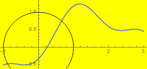
For multiple plots, use either command Show or you can use {} with commas. Show can be used to change the options of an existing graphic or to combine multiple graphics.
Show[{g1, Graphics[Circle[]]}, Background -> Yellow, AspectRatio -> Automatic]
Example:
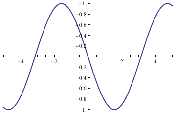
Plot sine function downward:
ListLinePlot[data1, PlotRange -> All];
ticks = Table[{-x, x}, {x, -5, 5, .2}];
ListLinePlot[{#, -#2} & @@@ data1, PlotRange -> {All, 1}, Ticks -> {All, ticks}, Axes -> True, PlotStyle -> Thick]
ListLinePlot[data1, PlotRange -> All];
ticks = Table[{-x, x}, {x, -5, 5, .2}];
ListLinePlot[{#, -#2} & @@@ data1, PlotRange -> {-1.3, 1.3},
Ticks -> {All, ticks}, Frame -> False, PlotRange -> All,
Epilog -> {Text["x", {5.5, 0}], Text["y", {0, -1.4}]},
PlotRangeClipping -> False, ImagePadding -> {{20, 20}, {20, 20}}]
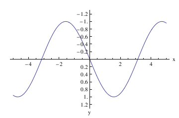
Now plot with arrows, but without units:
Graphics[Join[{Arrowheads[a]},
Arrow[{{0, 0}, #}] & /@ {{x, 0}, {0, y}}, {Text[
Style["x", FontSize -> Scaled[f]], {0.95*x, 0.1*y}],
Text[Style["y", FontSize -> Scaled[f]], {0.1 x, 1*y}]}]]
ListLinePlot[data1, PlotRange -> All];
ticks = Table[{-x, x}, {x, -5, 5, .2}];
Show[ListLinePlot[{#, -#2} & @@@ data1, PlotRange -> {-1.3, 0},
Ticks -> {None, None}, Frame -> False, PlotRange -> All,
PlotRangeClipping -> False, ImagePadding -> {{20, 20}, {20, 20}}],
axes[5.3, -1.33, .06, .05], Axes -> False]
Example: A Tractrix (from the Latin verb "trahere" -- pull, drag; plural: tractrices) is the curve along which an object moves, under the influence of friction, when pulled on a horizontal plane by a line segment attached to a tractor (pulling) point that moves at a right angle to the initial line between the object and the puller at an infinitesimal speed. By associating the object with a dog, the string with a leash, and the pull along a horizontal line with the dog's master, the curve has the descriptive name hundkurve (dog curve) in German. It is therefore a curve of pursuit. It was first introduced by Claude Perrault (1613--1688) in 1670. Trained as a physician, Claude was invited in 1666 to become a founding member of the French Academie des Sciences, where he earned a reputation as an anatomist. The first known solution was given by Christiaan Huygens (1692), who also named the curve the tractrix. Its parametric equation is
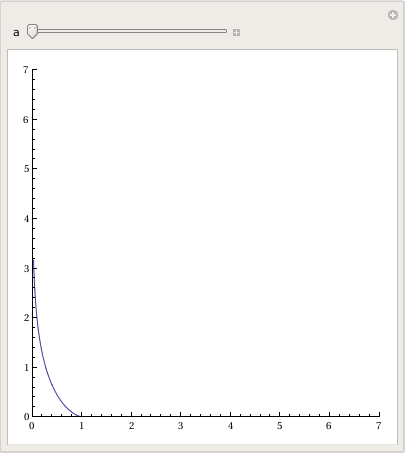
To plot tractrix curve, we use the following code which utilizes the Manipulate function:
Manipulate[
ParametricPlot[tractrix[a][t] // Evaluate, {t, 0, .99*\[Pi]},
PlotRange -> {0, 7}], {a, 1, 6}]
Export["tractrix1.gif",%]
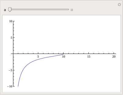
Plot[y'[x] = -Sqrt[a^2 - x^2]/x, {x, 0, 20},
PlotRange -> {-10, 10}], {a, 0, 20}]
a Log[x] + a Log[a^2 + a Sqrt[a^2 - x^2]]]}}
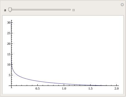
Plot[-Sqrt[a^2 - x^2] + a Log[a] - a Log[a^2] - a Log[x] + a Log[a^2 + a Sqrt[a^2 - x^2]], {x, 0, 20}, PlotRange -> All], {a, 1, 20}]
Plotting dots can be acomplished with a special subroutine:
- Visualization Mathematica Tutorial by John Boccio
- Plotting with Mathematica
- 2D Graphs by Michael A. Morrison
- Color Function by B G Higgins
Return to Mathematica page
Return to the main page (APMA0330)
Return to the Part 1 (Plotting)
Return to the Part 2 (First Order ODEs)
Return to the Part 3 (Numerical Methods)
Return to the Part 4 (Second and Higher Order ODEs)
Return to the Part 5 (Series and Recurrences)
Return to the Part 6 (Laplace Transform)
Return to the Part 7 (Boundary Value Problems)