Return to computing page for the second course APMA0340
Return to Mathematica tutorial for the first course APMA0330
Return to Mathematica tutorial for the second course APMA0340
Return to the main page for the course APMA0330
Return to the main page for the course APMA0340
Return to Part IV of the course APMA0330
Glossary
Nonlinear Equations
When we try to describe the world around us and ourselves, it turns out that the corresponding models are inherently nonlinear. The simplest experiment illustrating this observation is an attempt to bend a plastic beam. As long as the load is small, the deflection of the beam is approximately follows Hooke's law. But at some sufficiently large level the beam will simply deform or break. This strong and definitely irreversible change is an elementary example of nonlinear behavior illustrates an important feature enforcing us to formulate the first statement more precisely. The world is nonlinear, however, in many cases, if we consider only small influences and changes, the linear approximation is often sufficient to understand, predict, and control its behavior.
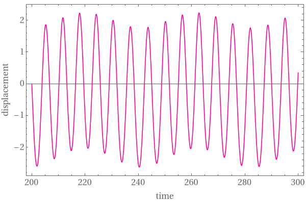
Suppose that an eardrum is being driven by a time(t)-dependent sinusoidal pressure wave. Suitably normalized and with arbitrary parameter values, the nonlinear ODE for the eardrum displacement y(t) from equilibrium is of the form
sol = NDSolve[{ode, y[0] == 2, y'[0] == -0.1}, y, {t, 200, 300}, MaxSteps -> 5000, Method -> "ExplicitRungeKutta", AccuracyGoal -> 10, PrecisionGoal -> 10]
Plot[Evaluate[y[t] /. sol], {t, 200, 300}, PlotPoints -> 1000, Frame -> True, PlotStyle -> Hue[0.9], FrameLabel -> {"time", "displacement"}, ImageSize -> {600, 400}, FrameTicks -> {{350, 500}, {-2, 0, 2}, {}, {}}, LabelStyle -> {FontFamily -> "Times", FontSize -> 16}]
|
|
|
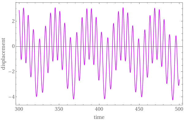
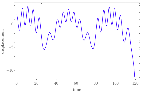
| Graph of the solution under the force \( 0.25\,\sin \left( 0.15\,t \right) \) | Graph of the solution under the force \( 1.25\,\sin \left( 0.15\,t \right) \) | Graph of the solution under the force \( 2.25\,\sin \left( 0.15\,t \right) \) |
|
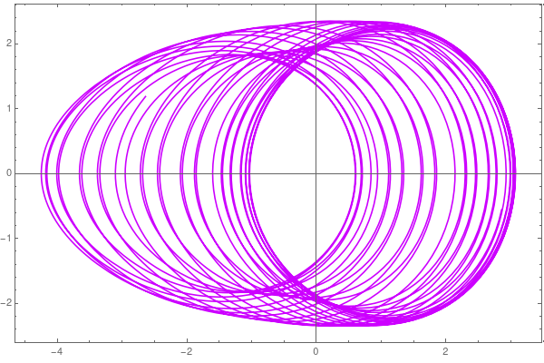
|
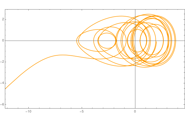
|
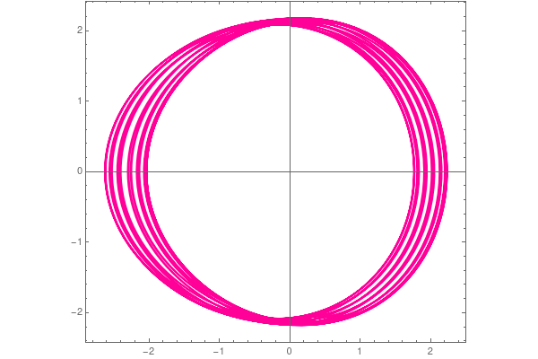
| Parametric plot v vs y under the force \( 0.25\,\sin \left( 0.15\,t \right) \) | Parametric plot v vs y under the force \( 1.25\,\sin \left( 0.15\,t \right) \) | Parametric plot v vs y under the force \( 2.25\,\sin \left( 0.15\,t \right) \) |
- Nayfeh, A.H. and Mook, D.T., Nonlinear Oscillations, Wiley, New York, 1979.
Return to Mathematica page
Return to the main page (APMA0330)
Return to the Part 1 (Plotting)
Return to the Part 2 (First Order ODEs)
Return to the Part 3 (Numerical Methods)
Return to the Part 4 (Second and Higher Order ODEs)
Return to the Part 5 (Series and Recurrences)
Return to the Part 6 (Laplace Transform)
Return to the Part 7 (Boundary Value Problems)