Preface
This tutorial was made solely for the purpose of education and it was designed for students taking Applied Math 0330. It is primarily for students who have very little experience or have never used Mathematica and programming before and would like to learn more of the basics for this computer algebra system. As a friendly reminder, don't forget to clear variables in use and/or the kernel. The Mathematica commands in this tutorial are all written in bold black font, while Mathematica output is in normal font.
Finally, you can copy and paste all commands into your Mathematica notebook, change the parameters, and run them because the tutorial is under the terms of the GNU General Public License (GPL). You, as the user, are free to use the scripts for your needs to learn the Mathematica program, and have the right to distribute this tutorial and refer to this tutorial as long as this tutorial is accredited appropriately. The tutorial accompanies the textbook Applied Differential Equations. The Primary Course by Vladimir Dobrushkin, CRC Press, 2015; http://www.crcpress.com/product/isbn/9781439851043
Return to computing page for the second course APMA0340
Return to Mathematica tutorial for the second course APMA0340
Return to the main page for the course APMA0330
Return to the main page for the course APMA0340
Return to Part II of the course APMA0330
Glossary
Landau Theory of Phase Transitions
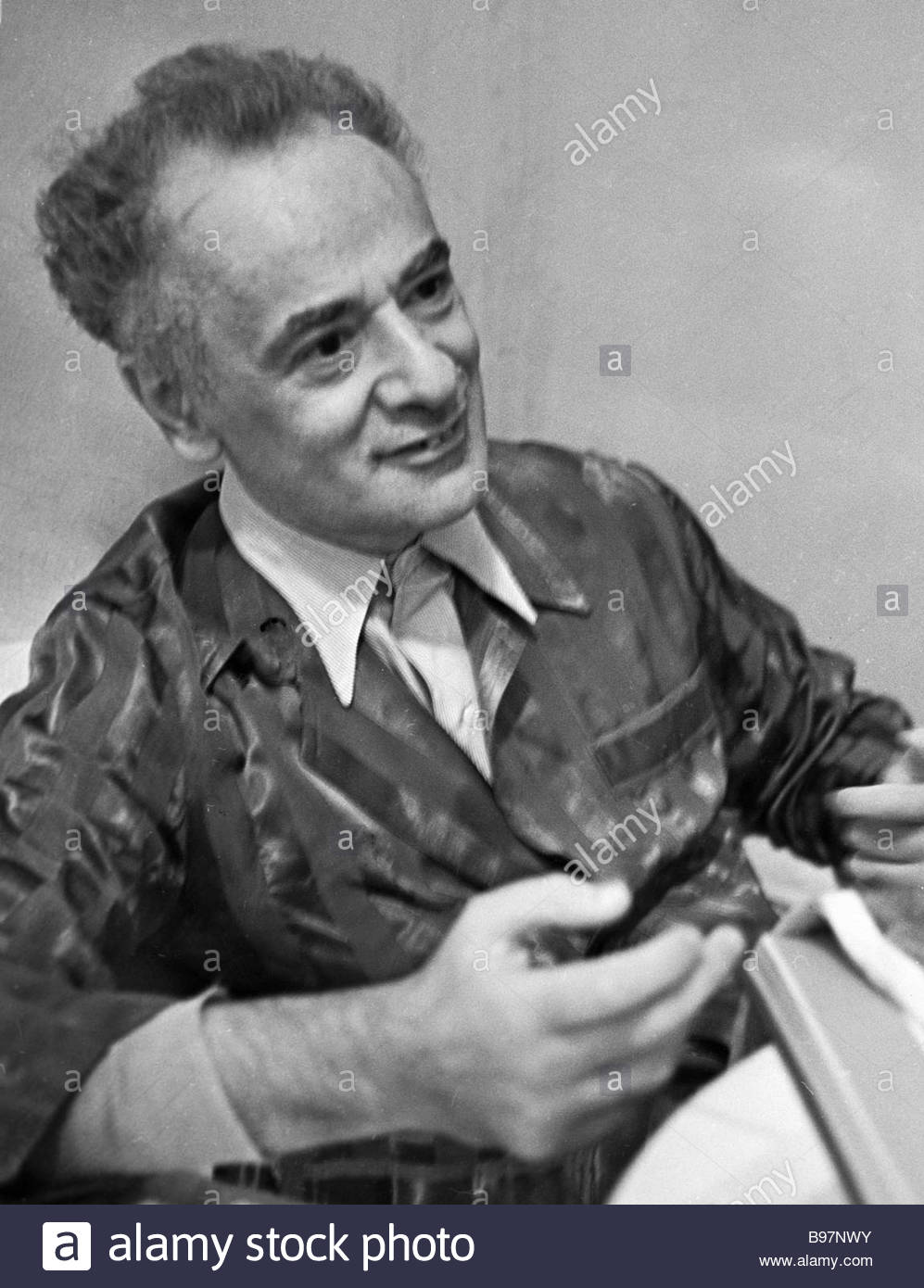
Lev Davidovich Landau (1908--1968) was a Soviet/Russian physicist who made fundamental contributions to many areas of theoretical physics. He received the 1962 Nobel Prize in Physics for his development of a mathematical theory of superfluidity that accounts for the properties of liquid helium II at a temperature below 2.17 K.
In 1924, he moved from Baku, where he was born to Jewish parents, to the main centre of Soviet physics at that time: the Physics Department of Leningrad State University. He received a doctorate in Physical and Mathematical Sciences in 1934. He was fired from St. Petersburg University for failing all students who, in his opinion, did not understand physics. Therefore, between 1932 and 1937 he headed the Department of Theoretical Physics at the National Scientific Center Kharkov Institute of Physics and Technology and lectured at the University of Kharkov and the Kharkov Polytechnical Institute. Landau developed a famous comprehensive exam called the "Theoretical Minimum" which students were expected to pass before admission to the school. During 27 years, only 43 candidates passed, but those who did later became quite notable theoretical physicists.
Phase transitions is an ubiquitous topic that includes magnets, liquid crystals, superconductors, crystals, amorphous equilibrium solids, and liquid condensation. These transitions occur between equilibrium states as functions of temperature, pressure, magnetic field, etc. A familiar example of such phase transition is water-vapor phase transition. We know the water does not immediately turn into vapor. At a boiling point we are facing a mixture (coexistence) of both phases involved. Liquid phase does not vanish until we provide sufficient amount of energy (heat). Another example gives transition of a disordered water/liquid into a crystalline solid when non apparent structure undergoes a transition to a structure with long range periodic order. Finally, one of the most common phase transitions from every day life is phase separation, which makes it necessary to shake the salad dressing. A phase transition occurs when the equilibrium state of a system changes qualitatively as a function of externally imposed constraints. These constraints could be temperature, pressure, magnetic field, concentration, degree of crosslinking, or any number of other physical quantities.
It is clear that transition between phases possessing different symmetries (e.g. distinct crystal modifications) cannot occur in a continuous manner. Our system will always be found in a state that reflects either one symmetry properties or another. In crystals, a transition between two different modifications can always take place after sudden rearrangement of its constituents, which would result in a discontinuous change of the state. Nonetheless there exist another type of transition affecting only the symmetry properties. Note that in such case there is no discontinuous change in the state of the system, i.e. positions of atoms are changing continuously, but there is a discontinuity in the symmetry at transition point.
To mathematically describe a transition, it is convenient to introduce a quantity called order parameter. In particular, we are interested in a quantity that takes a non-zero value below the critical point and exactly vanishes at the critical point, in the high-symmetry phase. For example, at a critical point, the magnetization is continuous -- as the parameters are tuned closer to the critical point, it gets smaller, becoming zero at the critical point. However, experiments on the liquid-gas phase transition and on three-dimensional magnets both point that even though the magnetization is continuous, its derivative is not.
The first major step toward theoretical understanding came from Landau (1937), and his approach is still called today Landau theory. His paper contains some typos and it took several decades for Nobel Prize winner in Physics 1982 Kenneth G. Wilson (1936--2013) and others to figure out how to fix it. It is important to emphasize that Landau’s original (genius) idea for an effective theory was and remains completely correct. It’s just that the naive computations do not give the right answers. Landau theory is an effective theory of the order parameter. To be precise about it, one first decides what the appropriate order parameter is to describe the phase transition. In one phase, the order parameter is non-vanishing, in another it vanishes. The basic assumption of Landau theory is that at a fixed value of the order parameter, the free energy as a function of the order parameter is analytic. The non-analyticity at a phase transition then comes because in the partition function one must sum over all possible values of the order parameter.
Landau’s theory of phase transitions is based on an expansion of the free energy of a thermodynamic system in terms of an order parameter, which is nonzero in an ordered phase and zero in a disordered phase. For example, the magnetization M of a ferromagnet in zero external field but at finite temperature typically vanishes for temperatures T > Tc, where Tc is the critical temperature, also called the Curie temperature in a ferromagnet. A low order expansion in powers of the order parameter is appropriate sufficiently close to Tc, i.e., at temperatures such that the order parameter, if nonzero, is still small.
With Landau’s assumption at fixed value of the order parameter is analytic, the free energy can be expanded in a Taylor series around the critical point. The symmetries of the theory determine the form of this expansion. The simplest example is the quartic free energy,
The phase transition of chocolate
As is well known, chocolate is a common foodstuff in daily life, as well as an important industrial material. For example, it is used as the raw material for a recent 3D food printer. the main ingredient in chocolate is cocoa butter, which has six crystalline states with different melting points. The crystalline state is related to the chemical composition of the cocoa butter, which, in turn, depends on the country of production and the harvest period. Therefore, the polymorphism of cocoa butter renders chocolate a complex structure.
- Rullong Ren et al, Hysteresis in the phase transition of chocolate, European Journal of Physics, 37, 2016.
- http://iypt.org/Tournaments/Shrewsbury
- Loisel C., Keller G., Bourgaux C., and Ollivon M. Phase transition and polymorphism of cocoa butter. Journal of the American Oil Chemists' Society, 75, issue 4, 425--439, 1998.
- Yeomans J.M., Statistical Mechanics of Phase Transitions, New York, Clarendon, 1992.
- Dovonshire A.F., Theory of ferroelectrics. Advances in Physics, 3, no. 10, 85--130, 1954.
Chocolate is usually solid at room temperature (20oC -- 25oC) and melts when the temperature rises to body temperature (36oC -- 37.5oC); that is, the phase transition occurs during solidification and melting. in the re-cooling process, however, chocolate remains a liquid when the temperature drops to room temperature (so it exhibits hysteresis). In fact, hysteresis behaviors widely exist in the phase transitions for ferromagnetic or ferroelectric materials.
According to Landau theory, the free energy of the system can be expressed as
Return to Mathematica page
Return to the main page (APMA0330)
Return to the Part 1 (Plotting)
Return to the Part 2 (First Order ODEs)
Return to the Part 3 (Numerical Methods)
Return to the Part 4 (Second and Higher Order ODEs)
Return to the Part 5 (Series and Recurrences)
Return to the Part 6 (Laplace Transform)
Return to the Part 7 (Boundary Value Problems)