Return to computing page for the first course APMA0330
Return to computing page for the second course APMA0340
Return to computing page for the fourth course APMA0360
Return to Mathematica tutorial for the first course APMA0330
Return to Mathematica tutorial for the second course APMA0340
Return to Mathematica tutorial for the fourth course APMA0360
Return to the main page for the course APMA0330
Return to the main page for the course APMA0340
Return to the main page for the course APMA0360
Return to Part VI of the course APMA0330
is said to be the Laplace transform of f provided that the integral \eqref{EqLaplace.1} converges for some value
\( \lambda = s \) of a parameter λ. Therefore, the Laplace transform of a function
(if it exists) depends on a parameter λ, which could be either a real number or a complex number. Saying that
a function f(t) has a Laplace transform fL means that for some λ = s, the limit
exists. From the definition of integral, it follows that the Laplace transform
does not depend on the values of an integrated function at a discrete number
of points. Therefore, the Laplace transform can map different functions into
the same output. Since application of the Laplace transformation to
differential equations requires the inverse Laplace transform, we need a
class of functions that is in bijection relation with its Laplace transforms.
The integral that defines the Laplace transform does not have to
converge. For example, neither \( {\cal L} \left[ 1/t \right] \) nor
\( {\cal L} \left[ e^{t^2} \right] \) exist.
There are known some sufficient conditions
guaranteeing the existence of \( {\cal L} \left[ f(t) \right] . \)
Theorem 1:
If a function f is absolutely integrable over any finite interval from
\( [0, \infty ) ; \) and the Laplace integral \( \int_0^{\infty} f(t)\,e^{-\lambda t} \,{\text d} t \)
converges for some complex number
\( \lambda = s , \) then it converges in the
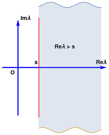
half-plane \(
\mbox{Re}\,\lambda > \mbox{Re}\, s , \)
i.e., in \( \left\{ \lambda \in \mathbb{C} \, : \, \Re\,
\lambda > \Re\, s \right\} . \)
Definition:
The smallest real number σ∈ℝ for which the integral \( \int_0^{\infty} f(t)\,e^{-\sigma t} \,{\text d} t \)
converges is called the abscissa of convergence of the function f.
We plot the abscissa of convergence and the domain where the Laplace transformation converges.
Abscissa of convergence and the domain of convergence for a Laplace transformation.
Mathematica code
Theorem 2: The Laplace transform is a linear operator.
In most applications t is the time and the domain of the real variable
t is the time domain. But the product λt in
\( e^{-\lambda\, t} \) is necessarily a pure number. One way to see this is by expanding the exponential function into the Taylor series
If λt had any units, such as millimeters or seconds, the terms in the series would all have different units and summation would make no sense. Since λt is a pure number, λ must have the units of 1/t. Hence, the product λt represents a dimensionless number (such as cycles) and λ has the units of frequency. It is often advantageous to let λ be complex, and consider it as the complex frequency. Then the set of values of λ is referred to as the frequency domain.
Definition: A function f is said to be piecewise continuous or intermittent on a finite closed interval [𝑎,b] if
the interval can be divided into finitely many subintervals so that f(t) is continuous on each subinterval and
approaches a finite limit at the end points of each subinterval from the interior.
A function is said to be piecewise continuous or intermittent on the infinite interval if it is piecewise continuous on every finite compact subinterval.
For our needs, we will use more restrictive definition of the intermittent function.
A function f(t), defined on semi-infinite interval [0, ∞), is piecewise continuous if this interval can be broken into finite number of pieces
so that the function f(t) is continuous on each of them and has finite limit values at the endpoints. A piecewise continuous function can be defined as
where each function fk(t), k = 1, 2, … , m, is continuous on the interval (𝑎k, bk) and has finite limit values at 𝑎k and
bk.
We do not specify the values of the function f(t) at endpoints
(𝑎k, bk) because we are going to apply the Laplace transformation to such intermittent functions; recall that the integral is not sensitive to the values of the function at a finite number of points. So wherever the function has values at the points of discontinuities, its Laplace transform does not depend on these values.
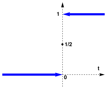
Definition: The
Heaviside functionH(t) is the unit step function:
It is known in calculus that if a function f is intermittent on a finite closed (compact) interval, then it is integrable on that interval. But for integrability of the product \( f(t)\, e^{-\lambda t} \) on the semi-infinite interval [0, ∞), we need a stronger condition than piecewise continuity. The following definition provides a sufficient condition on the function f to possess the Laplace transform.
Definition:
A function \( f(t), \ t \in [0, \infty ) \) is said to be a function-original
if it has a finite number of points of discontinuity (finite jumps) on every finite subinterval of
\( [0, \infty ) \) and it grows not faster than an exponential, that is
with some constants c, M, and T. Moreover, we assume that at points of discontinuity the
values of a function-original are equal to the corresponding mean values:
The Laplace transform of such a function is called the image.
In practical applications, the mean value property \eqref{EqLaplace.4} is not essential---it is used mostly in theoretical analysis. We usually do not pay attention to values of the function-original at the points of discontinuity (if any). However, be aware that the inverse Laplace transformation (as well as Fourier) restores the function with the mean value property. Therefore, the inverse Laplace transform automatically defines a function that has the property \eqref{EqLaplace.4}.
Definition:
We say that a function f is of exponential order if the inequality \( | f(t) | \le M\, e^{ct} \) holds for some constants
c, M, and T. We abbreviate this as
\( f = O\left( e^{ct} \right) \) or
\( f \in O\left( e^{ct} \right) . \)
A function f is said to be of exponential order α, or
eo(α) for abbreviation, if
\( f = O\left( e^{ct} \right) \) for any real number c > α, but not when
c < α.
Theorem 3: The Laplace transform exists for a function of exponential order, and tends to zero at infinite point.
Theorem 4: The Laplace transform establishes a one-to-one correspondence between
functions-originals and their images. ⧫
Examples
Example 1:
The Laplace transforms of the unit function and the Heaviside function are the same and equal to
where \( \Gamma (\nu ) = \int_0^{\infty} t^{\nu -1} \, e^{-t} \, {\text d} t \) is the Gamma-function of Euler.
Let us consider a particular case when p = -½.
The function has infinite discontinuity at t = 0. Hence, this function is not piecewise continuous on [0, ∞). However, its Laplace transform exists and can be found by
substitution λt = x², which gives
Note that the Laplace transform of the power function tp (t ≥ 0) exists only when p > -1. Otherwise, the Laplace transform does not exist because the corresponding integral diverges.
This example shows that the Laplace transform exists for a wider class of functions than functions-original.
■
Example 3:
The Laplace transform of the exponential function is
Example 4:
To find the
Laplace transform of the trigonometric functions, we recall that they are
real and
imaginary parts of pure imaginary exponential functions (known as Euler's formula):
where j is the unit vector in positive vertical direction on the complex plane, so j2 = -1. As usual, ℑ = Im is the imaginary part of a complex number; correspondingly, ℜ = Re is the real part of a complex number. So ℑ(𝑎 + jb) = b and ℜ(𝑎 + jb) = 𝑎.
Let us take 𝑎 in Eq.(4.1) to be pure imaginary, so 𝑎 ↦ j𝑎. Then
Here ℜ denotes the real part of a complex number, so ℜ(𝑎 + jb) = 𝑎, and ℑ is the imaginary part, so ℑ(𝑎 + jb) = b. The abscissa of convergence for these trigonometric functions is zero. Note that tangent function does not have a Laplace transform because the corresponding integral \eqref{EqLaplace.1} diverges.
Finally, we present some examples of Mathematica codes involving the Laplace transform.
Example 5:
We present some examples to show how Mathematica can be helpful in dealing with Laplace transformation and its applications. We start with t4sin(𝑎t):
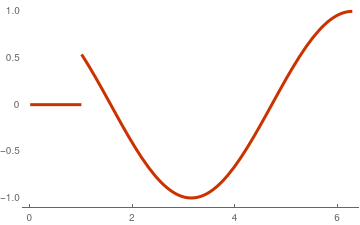
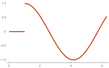
There are two kinds of delayed functions. Let us consider a familiar trigonometric function: cos(t). We construct from it two delayed functions: f(t) = cos(t)H(t−𝑎)
and g(t) = cos(t−𝑎)H(t−𝑎).
You will learn in section iv how to handle this case; however, we want to demonstrate the power of Mathematica in determination of the Laplace transform for complicated functions.
Return to Mathematica page
Return to the main page (APMA0330)
Return to the Part 1 (Plotting)
Return to the Part 2 (First Order ODEs)
Return to the Part 3 (Numerical Methods)
Return to the Part 4 (Second and Higher Order ODEs)
Return to the Part 5 (Series and Recurrences)
Return to the Part 6 (Laplace Transform)
Return to the Part 7 (Boundary Value Problems)