Preface
This tutorial was made solely for the purpose of education and it was designed for students taking Applied Math 0330. It is primarily for students who have very little experience or have never used Mathematica and programming before and would like to learn more of the basics for this computer algebra system. As a friendly reminder, don't forget to clear variables in use and/or the kernel. The Mathematica commands in this tutorial are all written in bold black font, while Mathematica output is in normal font.
Finally, you can copy and paste all commands into your Mathematica notebook, change the parameters, and run them because the tutorial is under the terms of the GNU General Public License (GPL). You, as the user, are free to use the scripts for your needs to learn the Mathematica program, and have the right to distribute this tutorial and refer to this tutorial as long as this tutorial is accredited appropriately. The tutorial accompanies the textbook Applied Differential Equations. The Primary Course by Vladimir Dobrushkin, CRC Press, 2015; http://www.crcpress.com/product/isbn/9781439851043
Return to computing page for the second course APMA0340
Return to Mathematica tutorial for the first course APMA0330
Return to Mathematica tutorial for the second course APMA0340
Return to the main page for the course APMA0330
Return to the main page for the course APMA0340
Return to Part II of the course APMA0330
Glossary
Plotting Solutions of ODEs
When Mathematica is capable to find a solution (in explicit or implicit form) to an initial value problem, it can be plotted as follows. Let us consider the initial value problem
a = DSolve[{y'[x] == -2 x y[x], y[0] ==1}, y[x],x];
Plot[y[x] /.a, {x,-2,2}]
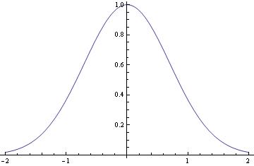
In this command sequence, I am first defining the differential equation that I want to solve. In this line, I define the equation
and the initial condition as well as the independent and dependent variables.
In the second line, I am commanding Mathematica to evaluate the given differential equation and plot its result. I then
command Mathematica to solve the equation and plot the given result of the initial value problem for the range listed above.
Typing these two commands together allows Mathematica to solve the initial value problem for you and to graph the initial
value problem's solution.
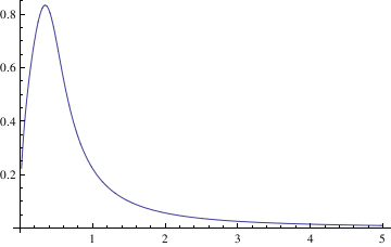
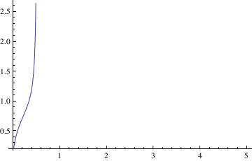
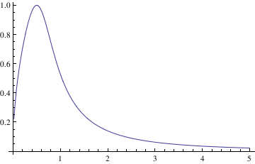
If you need to plot a sequence of solutions with different initial conditions, one can use the following script:
IC = {{0.5, 0.7}, {0.5, 4}, {0.5, 1}};
Do[ansODE[i] =
Flatten[DSolve[{myODE, y[IC[[i, 1]]] == IC[[i, 2]]}, y[t], t]];
myplot[i] = Plot[Evaluate[y[t] /. ansODE[i]], {t, 0.02, 5}];
Print[myplot[i]]; , {i, 1, Length[IC]}]
DSolve::bvnul: For some branches of the general solution, the given
boundary conditions lead to an empty solution. >>
 |
 |
 |
DSolve::bvnul: For some branches of the general solution, the given
boundary conditions lead to an empty solution. >>
In the above commands, you define the differential equation that you want to solve and the initial conditions (the respective variables are x and y). Flattening creates a list of the equations. Then you are asking Mathematica to evaluate the different equations according to their different initial conditions. Finally, the Print command tells Mathematica to plot the graphs and the size that you want the lines on the graphs to be.
When you enter these commands, you may receive a line saying that some of the branches lead to empty solutions, but this just means that DSolve cannot find a unique solution for part of the equation. However, this does not appear to affect the final graph.
To plot a family of solutions to
Clairaut's equation, we type:
samples1 = Table[f1[x], {c, -20/3, 8, 1}]
Plot[Evaluate[samples1], {x, -3, 3}, PlotStyle -> {Black}]
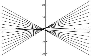
In this command, I am plotting a family of solutions to a differential equation. This command is not really any different from a normal plot command. The primary difference is that I have created a list of samples in a table. These samples have the variable c and then I can plug in different values of c to create the values in this table. This means that I am asking Mathematica to plot solutions with different values of the differential constant c. This command will plot a variety of different graphs over the range of c. The command on the second line also yields the different members of this family of equations associated with each value of c.
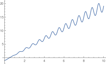
Usually, when Mathematica is capable to find a solution to the given initial value problem, it either present the solution via special functions or it takes too long to find it or even to give a negative answer that the solution is not available. We demonstrate this situation in the following example.
3\ \[Pi]\ K[1]]\), \(3\ \[Pi]\)]\)]\) \[DifferentialD]K[ 1]\)\) - 2 StruveL[0, 1/(3 \[Pi])])}}
Plot[y[x] /. nsol, {x, 0, 10}]
Return to Mathematica page
Return to the main page (APMA0330)
Return to the Part 1 (Plotting)
Return to the Part 2 (First Order ODEs)
Return to the Part 3 (Numerical Methods)
Return to the Part 4 (Second and Higher Order ODEs)
Return to the Part 5 (Series and Recurrences)
Return to the Part 6 (Laplace Transform)
Return to the Part 7 (Boundary Value Problems)