Preface
A differential equation, written in symmetric differential form \( M(x,y)\,{\text d}x + N(x,y)\,{\text d} y =0 , \) is exact if and only if there exists a potential function ψ such that its total differential is \( {\text d}\psi (x,y) = M(x,y)\,{\text d}x + N(x,y)\,{\text d} y . \)
Return to computing page for the second course APMA0340
Return to Mathematica tutorial for the second course APMA0340
Return to the main page for the course APMA0330
Return to the main page for the course APMA0340
Return to Part II of the course APMA0330
Glossary
Exact Equations
Recall the total differential of a function ψ(x,y) of two variables, denoted by dψ, is given by the expression
Let M(x,y) and N(x,y) be two smooth functions having continuous partial derivatives in some domain \( \Omega \subset \mathbb{R}^2 \) without holes. A differential equation, written in differentials
There are two approaches to find a potential function corresponding to an exact equation. The first one is based on integration of

|
Two contours of integrations along axeses.
line1 = Line[{{1, 0.5}, {4, 0.5}, {4, 3}}];
line2 = Line[{{1, 0.5}, {1, 3}, {4, 3}}]; a = {Graphics[{Thick, Dashed, Blue, line1}], Graphics[{Thick, line2}]} b = Graphics[Text[Style["(x,y)", FontSize -> 14, Red], {4.0, 3.2}]] b0 = Graphics[ Text[Style["(x0,y0)", FontSize -> 14, Blue], {1.0, 0.3}]] aa1 = Graphics[Arrow[{{1, 1}, {1, 2}}]] aa2 = Graphics[Arrow[{{2, 3}, {3, 3}}]] aa3 = Graphics[{Blue, Arrow[{{1, 0.5}, {3, 0.5}}]}] aa4 = Graphics[{Blue, Arrow[{{4, 1}, {4, 2}}]}] Show[aa1, aa2, aa3, aa4, a, b, b0, Axes -> True, AxesOrigin -> {0, 0}, PlotRange -> {{-0.5, 4.5}, {-0.5, 3.5}}, AxesLabel -> {x, y}, TicksStyle -> Directive[FontOpacity -> 0, FontSize -> 0]] |
|
| Two contours of integration. | Mathematica code |
If we integrate along black line (vertically where dx = 0 and then horizontally where dy = 0), we get
Now if we integrate along blue dashed line (horizontally where dy = 0 and then vertically where dx = 0), we get
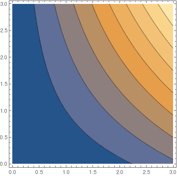
Example: The equation \( y \,\text{d}x + x \,\text{d}y =0 \) is exact because \( M_y =1 = N_x \) for \( M= y \quad\mbox{and} \quad N= x . \) Suppose that the initial condition \( y(2)=3 \) is given.
We type in Mathematica:
{p1, p2} = {2, 3};
Simplify[D[MM[x, y], y] == D[NN[x, y], x]]
Integrate[MM[x, p2], {x, p1, X}] + Integrate[NN[X, y], {y, p2, Y}]
The solution is psi[x,y]==0:
Define the gradient function:
and then check our potential function:
Example: Consider the differential equation
a=TrueQ[D[MM,y]==D[NN,x]];
If[a==True, Print["The equation is exact"], Print["The equation is not exact"]]
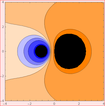
Example: An electrostatic potential built from a collection of point charges qi at positions ii
ElectroStaticPotential[{Subscript[q, 1], Subscript[q, 2]}, {{Subscript[x, 1], Subscript[y, 1]}, {Subscript[x, 2], Subscript[y, 2]}}, {x, y}] // TraditionalForm
|
Two charges q1 = -1 and q2 = 2
ContourPlot[
Evaluate[ElectroStaticPotential[{-1, 2}, {{-1, 0}, {1, 0}}, {x,
y}]], {x, -4, 4}, {y, -4, 4}, Contours -> {-0.75, -0.25, -0.1, 0, 0.1, 0.25, 0.75}, PlotRange -> 1, ClippingStyle -> Automatix, ContourShading -> c] |
|
| Electrostatic potential of two charges. | Mathematica code |
|
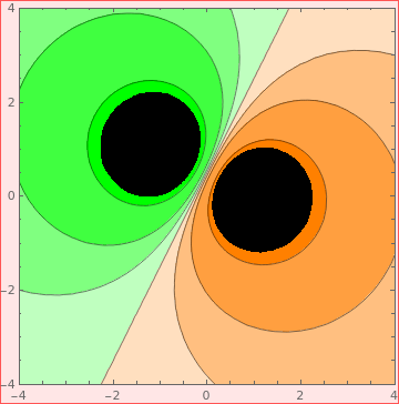
Three charges q1 = -1 and q2 = -1, and q3 = 2
ContourPlot[
Evaluate[ElectroStaticPotential[{-1, -1,
2}, {{-1, 1}, {-1, 1}, {1, 0}}, {x, y}]], {x, -4, 4}, {y, -4, 4}, Contours -> {-0.75, -0.25, -0.1, 0, 0.1, 0.25, 0.75}, PlotRange -> 1, ClippingStyle -> Automatix, ContourShading -> c] |
|
| Electrostatic potential of three charges. | Mathematica code |
■
Return to Mathematica page)
Return to the main page (APMA0330)
Return to the Part 1 (Plotting)
Return to the Part 2 (First Order ODEs)
Return to the Part 3 (Numerical Methods)
Return to the Part 4 (Second and Higher Order ODEs)
Return to the Part 5 (Series and Recurrences)
Return to the Part 6 (Laplace Transform)
Return to the Part 7 (Boundary Value Problems)