Functions

---

Since the Mathematica programming language (called the Wolfram language) is to a large extent a functional programming language, functions are the central objects here. The Wolfram Language has the most extensive collection of mathematical functions ever assembled. They can be accessed through the following web site:

A powerful tool of Mathematica is its ability to manipulate user-defined functions. This functions can be not only in terms of the internal build-in functions, but also in terms of procedures. To define a function, just type in the formula. We need to use a special form for the left hand side, which includes an underscore after the name of the variable, and a special "colon-equals" sign for the function definition:

There is no output on this input. To see it, type Print[f[x]] It is more appropriate to use Set(=) command You can use this function with different arguments or obtain its numerical values:

The symbol x_, pronounced ``x-blank,'' denotes a ``pattern'' named "x." For example, If one were to enter
f[x] =3*x+1, then f[3] and f[a+b] will not be evaluated, but g[x] will be evaluated because x is set as the only variable that this function will accept.
Function evaluation in Mathematica is indicated by square brackets. That is, while in mathematical notation, we write \( f(x), \) in Mathematica the correct syntax is f[x]. Ordinary parentheses are used exclusively for algebraic grouping. Thus we write (a*t) to indicate that the argument is the product of a and t. However, if f[x_]=3*x+1 is entered, then f[2] is 7, f[a+b] = 3a+3b+1, and f[x] is 3x+1 because entering x_ allows me to plug in different values for "x-blank."

To suppress output, type a semi-colon (;) at the end of input of your command. This is like how we suppress the result of a command by typing =; as was described earlier.

Function evaluation in Mathematica is indicated by square brackets. That is, while in mathematical notation, we write \( f(x), \) in Mathematica the correct syntax is f[x]. Ordinary parentheses are used exclusively for algebraic grouping. Thus we write (a*t) to indicate that the argument is the product of a and t.

The simplest user-defined functions are the "one-liners", where the quantity of interest can be computed by a single formula. However, in may cases, you may find it impossible to define the function's value in a single simple formula. Instead, you may need to carry out several steps of computation, using temporary variables. You may want several input values, and you may want the user to group some of those input values in curly brackets.

There are a few things to note when defining functions:

• Types of operations are expressed as + (addition), - (subtraction), *(multiplication), / (division). In Mathematica, you can use a blank space instead of typing * , so letter/numbers that are separated by space will be treated by Mathematica as multiplication.
• Exponents are expressed with carrots ^.
• Absolute values are expressed using the Abs[ ] command.
• Square roots (radicals) are expressed with the input Sqrt[ ] .
• When inputting π, you must type in Pi or \[Pi] .
• When using division, be sure to separate the numerators and denominators with parentheses to prevent errors.
• When you wish to substitute a variable with a value, use the option /.
• The % is a special symbol which takes in the most recently inputted equation. This is a useful symbol to use to avoid assigning equations to variables.
• If you want to determine the numerical value of a number, use N. The syntax is straightforward and simple:
  
  N[Pi]
  Out[1]= 3.14159

However, if you use the same command later, you will get

A function can also be defined analytically in another way. Say we want to define a cubic root function; then we type

The notion of a pure function comes from the calculus, and is widely used in functional programming languages, Mathematica in particular. From the practical viewpoint, the idea is that often we need some intermediate functions which we have to use just once, and we don't want to give them separate names. Pure functions allow their use without assigning them names, storing them in the global rule base etc. Another application of them is that while they can be assigned to some symbols, they exist independently of their arguments and can be called just by name with the arguments being supplied separately, so that the "assembly" to the working function happens already at the place where the function is used. Finally, these functions may be dynamically changed and modified during the program's execution.

Wolfram language allows one to define a pure function in which arguments are specified as #, #1, #2, etc. There are several equivalent ways to write pure functions in the Wolfram Language. The idea in all cases is to construct an object which, when supplied with appropriate arguments, computes a particular function. Thus, for example, if fun is a pure function, then fun[a] evaluates the function with argument a. There are some examples.

We start with defining a pure function that squares its argument:

and then rule-defined function To see their differences, use a special command DownValues[f] that gives a list of transformation rules corresponding to all downvalues defined for the symbol f. So we type There are two differences that immediately come to mind:

1. Functions with down values won't autocompile when you use them in Table, Map, Nest etc. so therefore they are less efficient when used that way.
2. Functions with down values may (in all likelihood will) cause a security warning when present in an embedded cumulative distribution function.

These two forms of functions may be similar on the surface, but they are very different in terms of the underlying mechanisms involved. In a sense, Function represents the only true (but leaky) functional abstraction in Mathematica. Functions based on rules are not really functions at all, they are global versions of replacement rules, which look like function calls.

One big difference is in the semantics of parameter-passing. For rules (and therefore functions based on rules), it is more intruding, in the sense that they don't care about the inner scoping constructs, while Function (with named arguments only) will care. Functions are more concise and generally faster but patterns are a lot more expressive. When you don't need the expressive power of patterns you should probably use functions.

Next we define a sum of squares with Map command:

Consider a function that takes the second element from the list: We check It is recommended to use SetDelayed to define a function in most cases. What will happen, if we use the Set (=) command instead of SetDelayed (:=), when defining a function? This depends on the state of global variables present or defined in the system at the given moment. Here is an example: The function works fine, but this is so only because by the moment of the definition, the variable x did not have any global value (no global rule was associated with it), and thus the right-hand side x² evaluated trivially (to itself) and was recorded in the rule for function f in this way. This is what happens when x has a value at the moment of assignment: We see that now any input expression, regardless of its structure, will be replaced by 25. This behavior is in full agreement with the principles of operation of Set ( = ) assignment operator. It allows the right-hand side of the definition to evaluate. This evaluation happens as usual, using the values for all global variables or expressions which exist in the system at the moment of the definition. Then Set uses the result of this evaluation as a right-hand side for the new global rule, associated with the left-hand side of the assignment. Since x had a global value 5, it was used in the calculation of the right-hand side, which then became the right-hand side of the global rule associated with function f (definition of f).

So, the conclusion is that in the majority of cases, functions must be defined with SetDelayed (:=) rather than Set (=). Since SetDelayeddoes not evaluate the right-hand side of an assignment, we are safe in this case. However, there are instances when Set operator is more appropriate to define a function. In particular, this happens when a function may be symbolically precomputed so that it is stored in a form which allows a more efficient computation.

For positive real inputs, the function h[x] always shows 0, but for negative inputs it is 1; so the function s[x]=1-h[x] is the Heaviside function: and we have Also

While Mathematica knows many standard functions, it does not use all equivalent relations. For instance, Mathematica does not know that

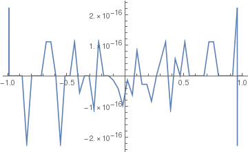
		ff[x_] = Simplify[ArcTanh[x] - (1/2)*Log[(1 + x)/(1 - x)]] ArcTanh[x] - 1/2 Log[(1 + x)/(1 - x)] Then we plot this function Plot[ff[x], {x, -1, 1}]
Graph of the function		Mathematica code

 

Consider a discontinuous function

First, we calculate some values:

We can calculate some values of function f simultaneously:

The derivative of the piecewise continuous function    f[t]:

 

Return to Mathematica page )
Return to the main page (APMA0330)
Return to the Part 1 (Plotting)
Return to the Part 2 (First Order ODEs)
Return to the Part 3 (Numerical Methods)
Return to the Part 4 (Second and Higher Order ODEs)
Return to the Part 5 (Series and Recurrences)
Return to the Part 6 (Laplace Transform)
Return to the Part 7 (Boundary Value Problems)