Preface


This section discusses differential equations involed in modeling fluid mechnics. we consider two such problems---Blasius equation and Jeffery--Hamel flow.

Return to computing page for the first course APMA0330
Return to computing page for the second course APMA0340
Return to Mathematica tutorial for the second course APMA0340
Return to the main page for the course APMA0330
Return to the main page for the course APMA0340
Return to Part VII of the course APMA0330
In this section we consider some boundary value problems from fluid mechanics---Blasius equation and Jeffery--Hamel flow.


Blasius and Sakiadis layers


A Blasius boundary layer (named after the German fluid dynamics physicist Paul Richard Heinrich Blasius, 1883--1970) describes the steady two-dimensional laminar boundary layer that forms on a semi-infinite plate which is held parallel to a constant unidirectional flow. Upon introducing a normalized stream function f, the Blasius equation becomes
\[ f''' + \frac{1}{2}\,f\,f'' =0 . \]
The boundary conditions are the no-slip condition:
\[ f(0) =0 , \qquad f' (0) =0, \qquad \lim_{y\to\infty} f' (y) = 1 . \]
In 1961 Sakiadis proposed another layer:
\[ f(0) =0 , \qquad f' (0) =1, \qquad \lim_{y\to\infty} f' (y) = 0 . \]
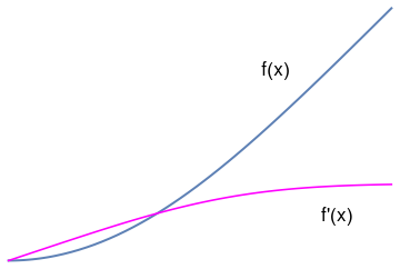
This is a nonlinear, boundary value problem (BVP) for the third order differential equation. The main obstacle in solving this problem numerically is request to evaluate f'(∞). Several strategies have been proposed in order to bypass this evaluation. One of them is to convert the given problem into the initial value problem, which was first achieved by K. Töpfer in 1912 by constructing a transformation of variables that reduces the BVP into an IVP. Actually, this leads to determination of the second derivative at the origin, f''(0), called the Blasius constant. Its numerical value was obtained by many researchers starting with K. Töpfer; however, the rigorous derivation of the Blasius constant is due to V.P. Varin in 2013 who obtained it in the form of a convergent series of rational numbers. Therefore, we assume that its value a = f′′(0) ≈ 0.33205733621 to be known (which is slightly less than 1/3). The knowledge of the Blasius constant is also necessary to evaluate the shear stress at the plate. Once this value is determined, we obtain the initial value problem, which can be solved numerically. So we solve the relevant initial value problem using different methods.

First, we start with Picard's iteration, and to achieve this we have two options: either to apply Picard's iteration directly to the third order Blasius equation directly or to convert it to a system of first-order differential equations. So we demonstrate both options, beginning with the latter.
blasius = NDSolve[{f'''[x] + 1/2*f[x]*f''[x] == 0, f[0] == 0, f'[0] == 0, f''[0] == 1/3}, f, {x, 0, 5}]
g = Plot[Evaluate[{f[x], f'[x]} /. blasius], {x, 0, 5}, PlotStyle -> {Thick, {Blue, Magenta}}]
txt1 = Graphics[ Text[Style["f(x)", FontSize -> 16, Black], {3.5, 2.5}]]
txt2 = Graphics[ Text[Style["f'(x)", FontSize -> 16, Black], {4.3, 0.6}]]
Show[txt1, txt2, g]


Picard's iteration applied to the third order equation


We use the fixed point formulation of the given initial value problem:

\[ f(x) = \frac{1}{6} - \frac{1}{4} \int_0^x \left( x-s \right)^2 f(s)\,f''(s) \,{\text d}s . \]
This leads to the following iteration procedure:
\[ y_{n+1} (x) = \frac{x^2}{6} - \frac{1}{4} \int_0^x \left( x-s \right)^2 y_n (s) \,y_{n}''(s) \,{\text d}s , \qquad n=3,4,\ldots , \]
with the following initial values:
\[ y_0 = 0, \quad y_1 =0, \quad y_2 = \frac{x^2}{6} . \]
For simplicity, we employ the Blasius constant to be 1/3. Next iteration results
y2[x_] = x^2 /6
y3[x_] = Simplify[ y2[x] - 1/4*Integrate[(x - s)^2*y2[s]*1/3, {s, 0, x}]]
-(1/216) x^2 (-36 + x^3)
\[ y_3 (x) = \frac{x^2}{216} \left( 36 - x^3 \right) . \]
We proceed with Mathematica.
(x^2 (23328 - 1296 x^3 + 198 x^6 - 5 x^9))/139968
y5[x_] = Simplify[ y4[x] - 1/4*Integrate[(x - s)^2*y4[x]*D[y4[x], x, x], {s, 0, x}]]
\[ f_5 (x) = \frac{x^2}{117546246144} \left( 19591041024 - 1632586752 x^3 + 498845952 x^6 - 154944576 x^9 + 16282944 x^{12} - 1518912 x^{15} + 82170 x^{18} - 1375 x^{21} \right) . \]
Now we plot the fifth approximation along with the numerical solution obtained by Mathematica.
Plot[{Evaluate[{f[x]} /. blasius], y5[x], f5[x]}, {x, 0, 2.4}, PlotStyle -> {Thick, {Blue, Orange, Magenta}}]
Therefore, we see that the two Picard's iteration procedures do not coincide and provide two different approximations. Moreover, the Picard's iteration applied directly to the third order equation converges much faster than the iteration based on reduction to the first order system of equations.

Example 3: Example. Consider the reduce Blasius equation for laminar flow over a flat plane:

\[ f''' (y) + f(y)\,f'' (y) =0 . \]
This equation is named after the German fluid dynamics physicist Paul Richard Heinrich Blasius (1883--1970), a student of Ludwig Prandtl (1875--1953), who provided a mathematical basis for boundary-layer drag. In 1908, Blasius solved the equation by using a series expansions method. In 1912, Toepfer solved the Blasius equation numerically by the application of the method of Runge and Kutta. In 1938, Howarth solved the Blasius equation more accurately by numerical methods and tabulated the result.

We convert the Blasius equation to a system of first order differential equations by setting

\[ u_1 = f, \quad f' = u_2 = \frac{{\text d}u_1}{{\text d}y} , \quad f'' = u_3 = \frac{{\text d}u_2}{{\text d}y} , \quad f''' = \frac{{\text d}u_3}{{\text d}y} . \]
Substituting these relations into the Blasius equation, we obtain
\[ \frac{{\text d}}{{\text d}y} \begin{bmatrix} u_1 \\ u_2 \\ u_3 \end{bmatrix} = \begin{bmatrix} u_2 \\ u_3 \\ - u_1 u_3 \end{bmatrix} . \]
This gives us an example of nonlinear autonomous vector equation with three unknowns.

Consider the initial value problem for the reduced Blasius equation

\[ f''' + \frac{1}{2}\, f\, f'' =0 , \qquad f(0) =0, \quad f' (0) = 0, \quad f'' (0) =1. \]
We set $u_1 = f$, $u_2 = f'$, and $u_3 = f''$; the the given Blasius equation can be written in vector form: \[ \frac{\text d}{{\text d}y} \begin{bmatrix} u_1 \\ u_2 \\ u_3 \end{bmatrix} = {\bf g} ({\bf u}) \equiv \begin{bmatrix} u_2 \\ u_3 \\ - \frac{1}{2} \, u_1 u_3 \end{bmatrix} . \] The initial iterative term is \[ {\bf \phi}_0 = \begin{bmatrix} 0 \\ 0 \\ 1 \end{bmatrix} . \] The first term becomes \[ {\bf \phi}_1 = \begin{bmatrix} 0 \\ 0 \\ 1 \end{bmatrix} + \int_0^y \begin{bmatrix} 0 \\ 1 \\ 0 \end{bmatrix} {\text d}y = \begin{bmatrix} 0 \\ y \\ 1 \end{bmatrix} . \] Next, \[ {\bf \phi}_2 (y) = \begin{bmatrix} 0 \\ 0 \\ 1 \end{bmatrix} + \int_0^y \begin{bmatrix} y \\ 1 \\ 0 \end{bmatrix} {\text d}y = \begin{bmatrix} y^2 /2 \\ y \\ 1 \end{bmatrix} , \] \[ {\bf \phi}_3 (y) = \begin{bmatrix} 0 \\ 0 \\ 1 \end{bmatrix} + \int_0^y \begin{bmatrix} y \\ 1 \\ - y^2 /4 \end{bmatrix} {\text d}y = \begin{bmatrix} y^2 /2 \\ y \\ 1-y^3 / 12 \end{bmatrix} , \] \[ {\bf \phi}_4 (y) = \begin{bmatrix} 0 \\ 0 \\ 1 \end{bmatrix} + \int_0^y \begin{bmatrix} y \\ 1- y^3 /12 \\ y^5 /48 \end{bmatrix} {\text d}y = \begin{bmatrix} y^2 /2 \\ y - y^4 /48 \\ 1+ y^6 /288 - y^3 /12 \end{bmatrix} . \] Therefore, we get the following Picard's iterations for $f(y)$: \[ \phi_0 = \phi_1 (y) = 0, \quad \phi_2 (y) = \phi_3 (y) = \phi_4 = y^2 /2 . \]     ■


Power Series Method


Adomian Decomposition Method (ADM)


text goes here


The ADM with accelerated Adomian polynomails


Jeffery--Hamel Flow


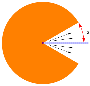
The Jeffery--Hamel flow is a flow created by a converging or diverging channel with a source or sink of fluid volume at the point of intersection of the two plane walls. It is named after George Barker Jeffery (1915--1957) and Georg Hamel (1917--1954), but it has subsequently been studied by many other scientists.

Consider two stationary plane walls with a constant volume flow rate is injected/sucked at the point of intersection of plane walls and let the angle subtended by two walls be 2 α. Take the cylindrical coordinate ( r , θ , z ) system with r = 0 representing point of intersection and θ = 0 the centerline and ( u , v , w ) are the corresponding velocity components. The resulting flow is two-dimensional if the plates are infinitely long in the axial z direction, or the plates are longer but finite, if one were neglect edge effects and for the same reason the flow can be assumed to be entirely radial i.e., u = u ( r , θ ), v = 0 , w = 0. Then the continuity equation and the incompressible Navier–Stokes equations reduce to

\begin{align*} \frac{\partial r\,u}{\partial r} &= 0 , \\ u\,\frac{\partial u}{\partial r} &= - \frac{1}{\rho}\,\frac{\partial p}{\partial r} + \nu \left[ \frac{1}{r}\,\frac{\partial }{\partial r} \left( r\,\frac{\partial u}{\partial r} \right) + \frac{1}{r^2} \, \frac{\partial^2 u}{\partial \theta^2} - \frac{u}{r^2} \right] , \\ 0 &= - \frac{1}{\rho\,r} \,\frac{\partial p}{\partial \theta} + \frac{2\nu}{r^2}\,\frac{\partial u}{\partial \theta} , \end{align*}
where u is the radial velocity, ρ is density, ν is the kinematic viscosity, p is fluid presure. The first equation tells us that r u(θ) = f(θ)
       
w = Graphics[{Orange, Disk[{0, 0}, 1, {Pi/6, 2*Pi - Pi/6}]}]
line = Graphics[{Blue, Thickness[0.01], Dashed, Line[{{0, 0}, {1.1, 0}}]}];
angle = Show[ ParametricPlot[#[[1]]*{Cos[\[Theta]], Sin[\[Theta]]}, {\[Theta], #[[2]], #[[3]]}, Axes -> False, PlotStyle -> #[[4]]] /. Line[x_] :> Sequence[Arrowheads[{-0.06, 0.06}], Arrow[x]] & /@ {{1, 0, Pi/6, Red}}]
txt = Graphics[ Text[Style["\[Alpha]", FontSize -> 16, Black], {1.1, 0.26}]];
ar1 = Graphics[Arrow[{{0.15, 0.05}, {0.7, 0.25}}]];
ar2 = Graphics[Arrow[{{0.15, 0.04}, {0.74, 0.12}}]];
ar3 = Graphics[Arrow[{{0.15, -0.04}, {0.74, -0.12}}]];
ar4 = Graphics[Arrow[{{0.15, -0.05}, {0.7, -0.25}}]];
p = Graphics[{PointSize[Large], Purple, Point[{0, 0}]}];
Show[w, angle, line, txt, ar1, ar2, ar3, ar4, p]
   Geometry of Jeffry--Hamel flow       Mathematica code

First, we note that the floow is symmetrical with respect to the centerline θ = 0, and we can consider the equation within the wedge 0 ≤ θ ≤ 1. Now by introducing the dimensionless variables

\[ F(\eta ) = \frac{f(\theta )}{f_{\max}} , \qquad\mbox{where}\quad 0 \le \eta = \frac{\theta}{\alpha} \le +1 , \]
and eliminating the pressure term, we derive the third order differential equation (after some simplifications)
\[ F''' + 2\,R_e\,\alpha \, F\,F' + 4\alpha^2 F' =0 . \]
The Reynolds number of flow is introduced as:
\[ R_e = \frac{f_{\max}}{\nu}\,\alpha , \]
where fmax is the velocity at the centerline of the channel, and α is the channel half-angle. The boundary conditions of the Jeffery-Hamel flow in terms of F(η) are expressed as follows:
\[ \begin{split} F(0) = 1, \quad F' (0) = 0 , \qquad\mbox{(at centerline)} , \\ F(1) =0 \qquad\mbox{at the upper body of channels.} \end{split} \]
It is convenient to represent the reduced Jeffry--Hamel equation in the operator form
\[ L[F] = N\left[ F\right] , \]
where
\[ L[F] = \texttt{D}^3 F = f''' \qquad \mbox{and} \qquad N\left[ F\right] = -2\,R_e\,\alpha \, F\,F' - 4\alpha^2 F' . \]

Picard's Iteration


Picard's iteration scheme defines the solution to the given boundary value problem
\[ \begin{split} L[F] \equiv \texttt{D}^3 F = f''' = N\left[ F\right] \equiv -2\,R_e\,\alpha \, F\,F' - 4\alpha^2 F' , \\ F(0) =1, \quad F' (0) =0, \quad F(1) =0 ; \end{split} \]
as the limit of the sequence of functions { yn(η) }, where each term is defined recursively by solving the boundary value problem:
\[ \begin{split} L\left[ y_{n+1} (\eta )\right] = N\left[ y_n (\eta) \right] , \\ y_{n+1} (0) = 1, \quad y'_{n+1} (0) =0, \quad y_{n+1}(1) =0 ; \quad n=0,1, \ldots . \end{split} \]
The initial term is chosen to satisfy the boundary condition as
\[ y_0 (\eta ) = 1 - \eta^2 . \]
The inverse operator
\[ L^{-1} \left[ f(x) \right] \equiv \texttt{D}^{-3} f(x) = \frac{1}{4} \, \int_0^x \left( x-t \right)^2 f(t)\,{\text d} t - \frac{1}{4} \, \int_x^1 \left( x-t \right)^2 f(t)\,{\text d} t + C_0 + C_1 x + C_2 x^2 \]
contains three arbitrary constants. To identify them, we use the boundary conditions:
LM[x_] = 1/4*Integrate[(x - t)^2 *f[t], {t, 0, x}] - 1/4*Integrate[(x - t)^2 *f[t], {t, x, 1}] + a + b*x + c*x^2 ;
Solve[{LM[0] == 1, LM[1] == 0, LM'[0] == 0}, {a, b, c}]
So
\[ L^{-1} \left[ f(x) \right] = \frac{1}{4} \, \int_0^x \left( x-t \right)^2 f(t)\,{\text d} t - \frac{1}{4} \, \int_x^1 \left( x-t \right)^2 f(t)\,{\text d} t + 1 + \frac{1}{4} \int_0^1 t^2 f(t) \,{\text d}t - \frac{x}{2} \int_0^1 t\,f(t)\,{\text d} t - x^2 \left( 1 + \frac{1}{4} \int_0^1 \left( 1 -4t + 2t^2 \right) f(t) \,{\text d}t \right) . \]
We check the answer with Mathematica:
IM[x_] = 1/4*Integrate[(x - t)^2 *f[t], {t, 0, x}] - 1/4*Integrate[(x - t)^2 *f[t], {t, x, 1}] + 1 +1/4*Integrate[t^2*f[t], {t,0,1}] -x/2 * Integrate[t*f[t], {t,0,1}] - x^2 *(1 + 1/4 * Integrate[(1 -4*t +2*t^2)*f[t], {t,0,1}] )
IM[0]
1
Simplify[IM[1]]
Simplify[(-1 + t)^2 - 2*t + t^2 - 1 - 2*t^2 + 4*t]
0
D[IM[x], x] /. x -> 0
0
D[IM[x], {x, 3}]
f[x]
Starting with y0(x) = 1 - x², we find the first term
f[x_]= 4*r*x*alpha*(1-x^2) + 8*x*alpha^2 ;
y1[x_] = 1/4*Integrate[(x - t)^2 *f[x], {t, 0, x}] - 1/4*Integrate[(x - t)^2 *f[x], {t, x, 1}] + 1 +1/4*Integrate[t^2*f[x], {t,0,1}] -x/2 * Integrate[t*f[x], {t,0,1}] - x^2 *(1 + 1/4 * Integrate[(1 -4*t +2*t^2)*f[x], {t,0,1}] )
Expand[%]
1 - x^2 - (4 alpha^2 x^3)/3 - 2/3 alpha r x^3 + (4 alpha^2 x^4)/3 + 2/3 alpha r x^4 + 2/3 alpha r x^5 - 2/3 alpha r x^6
So
\[ y_1 (x) = 1 - x^2 - \left( \frac{4\alpha^2}{3} + \frac{2\alpha\,R_e}{3} \right) \left( x^3 - x^4 \right) + \frac{2\alpha\,R_e}{3}\left( x^5 - x^6 \right) . \]
Next term we obtain similarly:
y1[x_] =1 - x^2 - (4 alpha^2 x^3)/3 - 2/3 alpha r x^3 + (4 alpha^2 x^4)/3 + 2/3 alpha r x^4 + 2/3 alpha r x^5 - 2/3 alpha r x^6 ;
f[x_] = Simplify[-2*r*alpha*y1[x]*y1'[x] - 4*alpha^2 *y1'[x]]
y2[x_] = 1/4*Integrate[(x - t)^2*f[t], {t, 0, x}] - 1/4*Integrate[(x - t)^2*f[t], {t, x, 1}] + 1 + 1/4*Integrate[t^2*f[t], {t, 0, 1}] - x/2*Integrate[t*f[t], {t, 0, 1}] - x^2*(1 + 1/4*Integrate[(1 - 4*t + 2*t^2)*f[t], {t, 0, 1}])
Expand[%]
1 - x^2 - (alpha^2 x^2)/3 - (4 alpha^4 x^2)/45 - 2/15 alpha r x^2 - 2/35 alpha^3 r x^2 + 2/945 alpha^5 r x^2 - ( 19 alpha^2 r^2 x^2)/1890 + (38 alpha^4 r^2 x^2)/31185 + ( 31 alpha^3 r^3 x^2)/162162 + (alpha^2 x^4)/3 + 1/6 alpha r x^4 + ( 4 alpha^4 x^5)/15 + 4/15 alpha^3 r x^5 + 1/15 alpha^2 r^2 x^5 - ( 8 alpha^4 x^6)/45 - 1/30 alpha r x^6 - 8/45 alpha^3 r x^6 - 2/45 alpha^2 r^2 x^6 - 8/63 alpha^3 r x^7 - 4/63 alpha^2 r^2 x^7 + 2/21 alpha^3 r x^8 - 2/63 alpha^5 r x^8 + 1/21 alpha^2 r^2 x^8 - 2/63 alpha^4 r^2 x^8 - 1/126 alpha^3 r^3 x^8 + 4/81 alpha^5 r x^9 + 1/54 alpha^2 r^2 x^9 + 4/81 alpha^4 r^2 x^9 + 1/81 alpha^3 r^3 x^9 - 8/405 alpha^5 r x^10 - 2/135 alpha^2 r^2 x^10 + 2/405 alpha^3 r^3 x^10 - 16/495 alpha^4 r^2 x^11 - 8/495 alpha^3 r^3 x^11 + 4/297 alpha^4 r^2 x^12 + 1/297 alpha^3 r^3 x^12 + 2/351 alpha^3 r^3 x^13 - 2/819 alpha^3 r^3 x^14
\[ \begin{split} y_2 (x) &= 1 - x^2 + \left( \frac{31\alpha^3 R_e^3}{162162} + \frac{38\alpha^4 R_e^2}{31185} - \frac{19 \alpha^2 R_e^2}{1890} + \frac{2\alpha^5\,R_e}{945} - \frac{2\alpha^3 R_e}{35} - \frac{2\alpha\,R_e}{15} - \frac{4\alpha^4}{45} - \frac{\alpha^2}{3} \right) x^2 \\ &\quad + \left( \frac{\alpha^2}{3} + \frac{\alpha\,R_e}{6} \right) x^4 + \left( 4\alpha^4 R_e + 4\alpha^3 R_e + \alpha^2 R_e^2 \right) \frac{x^5}{15} \\ &\quad - \left( \frac{8\alpha^3 R_e}{45} + \frac{2\alpha^2 R_e^2}{45} - \frac{\alpha\,R_e}{30} + \frac{8\alpha^4}{45} \right) x^6 - \left( \frac{8\alpha^3 R_e}{63} + \frac{4\alpha^2 R_e^2}{63}\right) x^7 + \left( \frac{2\alpha^3 R_e}{21} - \frac{2\alpha^5 R_e}{63} + \frac{\alpha^2 R_e^2}{21} + \frac{\alpha^2 R_e^2}{21} - \frac{2\alpha^4 R_e^2}{63} -\frac{\alpha^3 R_e^3}{126} \right) x^8 \\ &\quad + \cdots - \frac{2\alpha^3 R_e^3}{819}\, x^{14} . \end{split} \]
And then next:
y2[x_] = 1 - (12867 x^2)/11200 + x^3/6 - (23 x^5)/1200 + x^6/720 - x^8/20160 ;
f[x_] = Simplify[-2*r*alpha*y2[x]*y2'[x] - 4*alpha^2 *y2'[x]]
y3[x_] = 1/4*Integrate[(x - t)^2*f[t], {t, 0, x}] - 1/4*Integrate[(x - t)^2*f[t], {t, x, 1}] + 1 + 1/4*Integrate[t^2*f[t], {t, 0, 1}] - x/2*Integrate[t*f[t], {t, 0, 1}] - x^2*(1 + 1/4*Integrate[(1 - 4*t + 2*t^2)*f[t], {t, 0, 1}])
Expand[%]
Only a computer algebra system can handle all these operations, which is definetely not for humans.

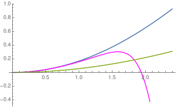
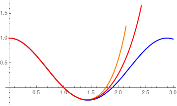
Now we plot this approximation along with the true solution, using Mathematica. First, to make our calculations exact, we set all parameters to be the integer, 1:

alpha=1; r=1;
Next plot contains the true graph in blue color and approximations y2(x) in orange and y3(x) in red.
s = NDSolve[{y'''[x] + 2*r*alpha*Times[y[x], y'[x]] + 4*alpha^2 *y'[x] == 0, y[0] == 1, y[1] == 0, y'[0] == 0}, y, {x, 0, 10}]
exact = Plot[{Evaluate[y[x] /. s]}, {x, 0, 3}, PlotRange -> All, PlotStyle -> {Thick, Blue}]
g2 = Plot[y2[x], {x, 0, 2.14}, PlotStyle -> {Thick, Orange}]
g3 = Plot[y3[x], {x, 0, 2.42}, PlotStyle -> {Thick, Red}]
Show[exact, g2, g3]
True solution (in blue) along with two approximations y2(x) in orange and y3(x) in red.


Adomian Decomposition Method (ADM)


We apply the Adomian decomposition method (ADM) to the problem written in operator form:

\[ L[F] = \texttt{D}^3 F = f''' = N\left[ F\right] = -2\,R_e\,\alpha \, F\,F' - 4\alpha^2 F' , \qquad F(0) =1, \quad F' (0) = F(1) =0. \]
According to the ADM, its solution is assumed to be in the infinte sum form:
\[ F(\eta ) = u_0 + u_1 + u_2 + \cdots = \sum_{n\ge 0} u_n , \]
where each term in this sum is obtained recursively
\[ L\left[ u_{n+1} \right] = A_n \left( u_0 , u_1 , \ldots , u_n \right) , \quad\mbox{subject to homogeneous boundary conditions}, \quad n=0,1,\ldots . \]
The initial term u0(x) = 1 - x² is the solution of
\[ L\left[ u_{0} \right] = 0, \qquad u_0 (0) =1, \quad u'_0 (0) =0, \quad u_0 (1) =0. \]
Here An are the Adomian polynomials:
\[ A_n \left( u_0 , u_1 , \ldots , u_n \right) = \left. \frac{1}{n!} \, \frac{{\text d}^n}{{\text d} \lambda^n} \, N \left[ \sum_{k\ge 0} \lambda^k u_k \right] \right\vert_{\lambda =0} , \quad n=0,1,2,\ldots . \]

We calculate the Adomian polynomials using Mathematica:

dvar[t_] = D[#, t] &
f[u_] = -2*r*alpha*Times[u[t], dvar[t][u[t]]] - 4*alpha^2 *dvar[t][u[t]]
u0[t_] = 1 - t^2
A0[t_] = ReplaceAll[f[u0], x -> t]
a0[t_] = 8 alpha^2 t + 4 alpha r t (1 - t^2)
LM[f_] = 1/4*Integrate[(x - t)^2*f[t], {t, 0, x}] - 1/4*Integrate[(x - t)^2*f[t], {t, x, 1}] + 1/4*Integrate[t^2*f[t], {t, 0, 1}] - x/2*Integrate[t*f[t], {t, 0, 1}] - x^2/4*Integrate[(1 - 4*t + 2*t^2)*f[t], {t, 0, 1}]
Expand[LM[a0]]
-(1/3) alpha^2 x^2 - 2/15 alpha r x^2 + (alpha^2 x^4)/3 + 1/6 alpha r x^4 - 1/30 alpha r x^6
So
\[ A_0 (t) = 4\,\alpha\, t \left( R_e + 2\alpha - R_e t^2 \right) . \]
To find the first term, we need to solve the boundary value problem:
\[ u''' (x) = A_0 (x) , \qquad u(0) = u' (0) =0 \quad\mbox{and} \quad u(1) =0 . \]
Of course, with Mathematica at hand, we accormplish this task without a problem. The inverse operator contains three arbitrary condtants
\[ L^{-1} \left[ f(x) \right] \equiv \texttt{D}^{-3} f(x) = \frac{1}{4} \, \int_0^x \left( x-t \right)^2 f(t)\,{\text d} t - \frac{1}{4} \, \int_x^1 \left( x-t \right)^2 f(t)\,{\text d} t + C_0 + C_1 x + C_2 x^2 \]
that we determine to satisfy the homogeneous boundary conditions.
lm[x_] = 1/4*Integrate[(x - t)^2 *f[t], {t, 0, x}] - 1/4*Integrate[(x - t)^2 *f[t], {t, x, 1}] + a + b*x + c*x^2
Solve[{lm[0] == 0, lm[1] == 0, lm'[0] == 0}, {a, b, c}]
So we get
\[ L^{-1} \left[ f(x) \right] \equiv \texttt{D}^{-3} f(x) = \frac{1}{4} \, \int_0^x \left( x-t \right)^2 f(t)\,{\text d} t - \frac{1}{4} \, \int_x^1 \left( x-t \right)^2 f(t)\,{\text d} t + \frac{1}{4} \int_0^1 t^2 f(t)\,{\text d}t -\frac{x}{2} \int_0^1 t\, f(t)\,{text d}t - \frac{x^2}{4} \int_0^1 \left( 1 -4t + 2t^2 \right) f(t)\,{\text d}t . \]
Now we define the needed operator L-1, which we denote as LM:
LM[f_] = 1/4*Integrate[(x - t)^2*f[t], {t, 0, x}] - 1/4*Integrate[(x - t)^2*f[t], {t, x, 1}] + 1/4*Integrate[t^2*f[t], {t, 0, 1}] - x/2*Integrate[t*f[t], {t, 0, 1}] - x^2/4*Integrate[(1 - 4*t + 2*t^2)*f[t], {t, 0, 1}]
NN[f_] = -2*r*alpha*Times[f[x], f'[x]] - 4*alpha^2 *f'[x]
u0[x_] = 1 - x^2
A0== NN[u0]
(* define the first term u1 *)
a0[t_] = 8 alpha^2 t + 4 alpha r t (1 - t^2)
LM[f_] = 1/4*Integrate[(x - t)^2*f[t], {t, 0, x}] - 1/4*Integrate[(x - t)^2*f[t], {t, x, 1}] + 1/4*Integrate[t^2*f[t], {t, 0, 1}] - x/2*Integrate[t*f[t], {t, 0, 1}] - x^2/4*Integrate[(1 - 4*t + 2*t^2)*f[t], {t, 0, 1}]
u1[t_]=Expand[LM[a0]]
8 alpha^2 x + 4 alpha r x (1 - x^2)
With the first Adomian polynomial in hand, we define the first term:
u1[x_] = -(1/3) alpha^2 x^2 - 2/15 alpha r x^2 + (alpha^2 x^4)/3 + 1/6 alpha r x^4 - 1/30 alpha r x^6
The first partial sum becomes
\[ \phi_1 (x) = u_0 (x) + u_1 (x) = 1- x^2 - \left( \frac{\alpha^2}{3} + \frac{2\alpha\,R_e}{15}\right) \left( x^2 - x^4 \right) - \frac{\alpha\,R_e}{30}\, x^6 . \]
We check our answer by solving the corresponding boundary value problem:
DSolve[{y'''[x] == 8 alpha^2 x + 4 alpha r x (1 - x^2) , y[0]==0 , y[1]==0, y'[0]==0}, y[x],x]
{{y[x] -> 1/30 (-10 alpha^2 x^2 - 4 alpha r x^2 + 10 alpha^2 x^4 + 5 alpha r x^4 - alpha r x^6)}}
\[ u_1 (x) = \frac{1}{30} \left[ 10 \alpha^2 x^4 + 4\alpha\, R_e \, x^4 - \alpha\,R_e x^6 - 10 \alpha^2 x^2 - 4\alpha\, R_e x^2 \right] . \]
Since the answer is the same, we move forward for calculating the second term. First, we need to build the corresponding Adomian polynomial:
\[ A_1 \left( u_0 , u_1 \right) = \left. \frac{1}{1!} \, \frac{{\text d}}{{\text d} \lambda} \, N \left[ \sum_{k\ge 0} \lambda^k u_k \right] \right\vert_{\lambda =0} = \left. - \frac{{\text d}}{{\text d} \lambda} \left[ 2\,R_e\,\alpha \left( u_0 + \lambda \, u_1 \right) \left( u'_0 + \lambda \, u'_1 \right) + 4\alpha^2 \left( u'_0 + \lambda \, u'_1 \right) \right] \right\vert_{\lambda =0} = - 2\,R_e\,\alpha \left( u_0 u'_1 + u'_0 u_1 \right) - 4\alpha^2 u'_1 . \]
We again ask Mathematica for help:
u0[x_] = 1 - x^2
u1[x_] = -(1/3) alpha^2 x^2 - 2/15 alpha r x^2 + (alpha^2 x^4)/3 + 1/6 alpha r x^4 - 1/30 alpha r x^6
f[x_] = -2*r*(Times[u0[x], u1'[x]] + Times[u0'[x], u1[x]]) - 4*alpha^2*u1'[x]
u2[x_] = Expand[1/4*Integrate[(x - t)^2*f[t], {t, 0, x}] - 1/4*Integrate[(x - t)^2*f[t], {t, x, 1}] + 1/4*Integrate[t^2*f[t], {t, 0, 1}] - x/2*Integrate[t*f[t], {t, 0, 1}] - x^2/4*Integrate[(1 - 4*t + 2*t^2)*f[t], {t, 0, 1}]]
Next, we determine the Adomian polynomialA2:
\[ A_2 \left( u_0 , u_1 , u2 \right) = \left. \frac{1}{2!} \, \frac{{\text d}^2}{{\text d} \lambda^2} \, N \left[ \sum_{k\ge 0} \lambda^k u_k \right] \right\vert_{\lambda =0} = \left. - \frac{{\text d}^2}{{\text d} \lambda^2} \left[ R_e\,\alpha \left( u_0 + \lambda \, u_1 + \lambda^2 u_2 \right) \left( u'_0 + \lambda \, u'_1 + \lambda^2 u'_2 \right) + 2\alpha^2 \left( u'_0 + \lambda \, u'_1 + u'_2 \right) \right] \right\vert_{\lambda =0} = - R_e\,\alpha \left( u_0 u'_2 + u_1 u'_1 + u'_0 u_2 \right) - 2\alpha^2 u'_2 . \]
Using Mathematica, we obtain
f[x_] = -r*(Times[u0[x], u2'[x]] + Times[u1'[x], u1[x]]+ Times[u0'[x], u2[x]]) - 2*alpha^2*u2'[x] ;
u3[x_] = Expand[1/4*Integrate[(x - t)^2*f[t], {t, 0, x}] - 1/4*Integrate[(x - t)^2*f[t], {t, x, 1}] + 1/4*Integrate[t^2*f[t], {t, 0, 1}] - x/2*Integrate[t*f[t], {t, 0, 1}] - x^2/4*Integrate[(1 - 4*t + 2*t^2)*f[t], {t, 0, 1}]];
      Finally, we plot these functions:
alpha = 1; r = 1;
y2[x_] = u0[x] + u1[x] +u2[x];
y3[x_] = y2[x] + u3[x];
s = NDSolve[{y'''[x] + 2*r*alpha*Times[y[x], y'[x]] + 4*alpha^2 *y'[x] == 0, y[0] == 1, y[1] == 0, y'[0] == 0}, y, {x, 0, 10}]
exact = Plot[{Evaluate[y[x] /. s]}, {x, 0, 3}, PlotRange -> All, PlotStyle -> {Thick, Blue}]
g2 = Plot[y2[x], {x, 0, 2.14}, PlotStyle -> {Thick, Orange}]
g3 = Plot[y3[x], {x, 0, 2.42}, PlotStyle -> {Thick, Red}]
Show[exact, g2, g3]
       True solution (in blue) along with two approximations y2(x) in orange and y3(x) in red.            Mathematica code


Accelerated Decomposition Method


The required solution is again the infinite sum
\[ F(\eta ) = u_0 + u_1 + u_2 + \cdots = \sum_{n\ge 0} u_n , \]
where each term in this sum is obtained recursively
\[ L\left[ u_{n+1} \right] = J_n \left( u_0 , u_1 , \ldots , u_n \right) , \quad\mbox{subject to homogeneous boundary conditions}, \quad n=0,1,\ldots . \]
The nonlinear operator N[F] is decomposed as
\[ N\left[ F \right] = J_0 + J_1 + J_2 + \cdots = \sum_{n\ge 0} J_n \left( u_0 , u_1 , \ldots , u_n \right) , \]
where
\[ J_n = N \left[ u_0 + u_1 + \cdots + u_n \right] - N \left[ u_0 + u_1 + \cdots + u_{n-1} \right] , \qquad J_0 = N\left[ u_0 \right] . \]
The initial term u,sub>0
for the ADM is the same as in GDM: u0 = 1 - η².


  1. S. Abbasbandy, A numerical solution of Blasius equation by Adomian’s decomposition method and comparison with homotopy perturbation method Chaos Solitons Fractals, 31 (2007), pp. 257-260
  2. S. Ahmad, A. M. Rohni, and I. Pop, “Blasius and Sakiadis problems in nanofluids [J],” Acta Mech. 218, 195–204 (2011). https://doi.org/10.1007/s00707-010-0414-6
  3. Aminikhah, Hossein, Analytical Approximation to the Solution of Nonlinear Blasius’ Viscous Flow Equation by LTNHPM, ISRN Mathematical Analysis Volume 2012, Article ID 957473, 10 pages http://dx.doi.org/10.5402/2012/957473
  4. Bataller, R.C., Numerical Comparisons of Blasius and Sakiadis Flows, MATEMATIKA, 2010, Volume 26, Number 2, pp. 187--196.
  5. Blasius, H., Grenzschichten in Flüssigkeiten mitkleiner Reibung, Zeitschrift für angewandte Mathematik und Physik (Journal of Applied Mathematics and Physics), 56:137, 1908.
  6. Solving the Blasius equation
  7. The Blasius equation, B. Bright, A. Fruchard, and T. Sari, 2010.
  8. Blasius equation
  9. A.J. Callegari, Nachman, Some singular nonlinear differential equations arising in boundary layer theory J. Math. Anal. Appl., 64 (1978), pp. 96-105
  10. Esmaili, Q., Ramiar, A., Alizadeh E., and Ganji, D.D., An approximation of the analytical solution of the Jeffery--Hamel flow by decomposition method, Physics Letters, A, 2008, 372, (19), 3434–3439. https://doi.org/10.1016/j.physleta.2008.02.006
  11. Fazio, R., Transformation methods for the Blasius problem and its recent variants, Proceedings of the World Congress on Engineering, 2008 Vol IIWCE 2008, July 2 - 4, 2008, London, U.K.
  12. Fraenkel, L. E., Laminar flow in symmetrical channels with slightly curved walls, I. On the Jeffery-Hamel solutions for flow between plane walls. Proceedings of the Royal Society of London. Series A. Mathematical and Physical Sciences, 1962, 267(1328), 119-138.
  13. Ganapol, B.D., Highly accurate solutions of the Blasius and Falkner--Skan boundary layer equations via convergence acceleration, University of Arizona
  14. Hamel, G., Spiralformige Bewegungen zaher Flussigkeiten, Jahresbericht der deutshen Math. Vereiniguug, 25 (1916), 34-60.
  15. He, J.-H., Approximate analytical solution of Blasius’ equation. Communications in σonlinear Science and Numerical Simulation, 3, 260-263 (1998).
  16. He, J.-H., A simple perturbation approach to Blasius equation. Applied Mathematics and Computation, 2003, Vol. 140, 217-222. https://doi.org/10.1016/s0096-3003(02)00189-3
  17. Jeffery, G.B., The two dimensional steady motion of a viscous fluid, Phil. Mag., 29 (1915), 455-465.
  18. Liao, S.J., An explicit, totally analytic approximate solution for Blasius’ viscous flow problems,  International Journal of Non-Linear Mechanics, 1999, 34(4). pp. 759--778.
  19. S. Liao, “An explicit, totally analytical approximate solution for Blasius equation [J],” Int. J. Non-Linear Mech. 34, 759–778 (1999). https://doi.org/10.1016/s0020-7462(98)00056-0
  20. S.J. Liao A challenging nonlinear problem for numerical techniques J. Comput. Appl. Math., 181 (2005), pp. 467-472
  21. Lin, J., A new approximate iteration solution of Blasius equation. Communications in Nonlinear Science and Numerical Simulation, 4, 91-94 (1999). https://doi.org/10.1016/s1007-5704(99)90017-5
  22. Lu, Z. and Law, C.K., “An iterative solution of the Blasius flow with surface gasification [J],” Int. J. Heat Mass Transfer 69, 223–229 (2014). https://doi.org/10.1016/j.ijheatmasstransfer.2013.10.020
  23. Mattioli, Franco, Blasius solution, University of Bologna, Italy.
  24. Parand, K., Dehghan, M., and Taghavi, A., Modified generalized Laguerre function Tau method for solving laminar viscous flow: The Blasius equation, Journal of Numerical methods for Heat & Fluid Flow, 2010, Vol. 20, Issue 7, pp.728--743, https://doi.org/10.1108/09615531011065539
  25. Prand, K., Dehghan, M., and Baharifard, F., “Solving a laminar boundary equation with the rational Gegenbauer functions [J],” Appl. Math. Mod. 37, 851–863 (2013). https://doi.org/10.1016/j.apm.2012.02.041
  26. Puttkammer, P.P., Boundary Layer over a Flat Plate, University of Twenter, 2013.
  27. Sakiadis, B. C. Boundary-layer behaviour on continuous Solid surfaces; boundary-layer equations for 2-dimensional and axisymmetric Flow, AIChE Journal, 1961, Vol. 7, Issue 1, pp. 26–28. https://doi.org/10.1002/aic.690070108
  28. Sakiadis, B. C. Boundary‐layer behavior on continuous solid surfaces: II. The boundary layer on a continuous flat surface, AIChE Journal, 1961, Vol. 7, Issue 2, pp. 221–225. https://doi.org/10.1002/aic.690070211
  29. Sari, M.R., kezzar, M., Adjabi, R., A comparison of Adomian and generalized Adomian methods in solving the nonlinear problem of flow in convergent-divergent channels, Applied Mathematical Sciences, 2014, Vol. 8, no. 7, pp. 321--336; http://dx.doi.org/10.12988/ams.2014.39495
  30. Schlichting, H. and Gersten, K., Boundary Layer Theory (8th revised and enlarged ed.), Springer-Verlag, Berlin, Heidelberg (2000)
  31. Töpfer, K., Bemerkung zu dem Aufsatz von H. Blasius: Grenzschichten in Flüssigkeiten mit kleinerReibung, Zeitschrift für angewandte Mathematik und Physik (Journal of Applied Mathematics and Physics), 60:397–398, 1912
  32. Treve, Y.M., On a class of solutions of the Blasius equation with applications, SIAM Journal of Applied Mathematics, 1967, Vol. 15, No. 5, 1209--1227. doi: 10.1137/0115103
  33. Varin, V.P., A solution of the Blasius problem, Keldysh Institute, Preprint No. 40, 2013.
  34. Wang, L. (2004), A new algorithm for solving classical Blasius equation, Applied Mathematics and Computation, 2004, Vol. 157 No. 1, pp. 1-9. https://doi.org/10.1016/j.amc.2003.06.011
  35. Weidman, P.D., Blasius boundary layer flow over an irregular leading edge, Physics of Fluids, 9, 1470 (1997); https://doi.org/10.1063/1.869268
  36. H. Weyl, “On the differential equations of the simplest boundary-layer problems [J],” Ann. Math. 43(2), 381–407 (1942). https://doi.org/10.2307/1968875
  37. Yu, L.-T. and Chen, C.-K., The solution of the Blasius equation by the Differential Transformation Method, Mathematical and Computer Modelling, 1998, Vol. 28, No. 1, pp. 101-111.
  38. B. Yao and J. Chen, “A new analytical solution branch for the Blasius equation with a shrinking sheet [J],” Appl. Math. Comp. 215, 1146–1153 (2009). https://doi.org/10.1016/j.amc.2009.06.057
  39. Yu, L.-T. and Chen, C.-K., Solutions of the Blasius equation by the differential transformation method, Mathematical Computaional Modeling, 28, No. 1, pp. 101--111, 1995.
  40. Zheng, J., Han, X., Wang, Z., Li, C., and Zhang, J., A globally convergent and closed analytical solution of the Blasius equation with beneficial applications, AIP Advances, Vol. 7, 065311 (2017); https://doi.org/10.1063/1.4985741


Return to Mathematica page
Return to the main page (APMA0330)
Return to the Part 1 (Plotting)
Return to the Part 2 (First Order ODEs)
Return to the Part 3 (Numerical Methods)
Return to the Part 4 (Second and Higher Order ODEs)
Return to the Part 5 (Series and Recurrences)
Return to the Part 6 (Laplace Transform)
Return to the Part 7 (Boundary Value Problems)