Preface


This section illustrates applications of the Adomian decomposition method (ADM for short) for numerical approximations of solutions to certain classes of nonlinear ordinary differential equations of first order. In layman's terms, as the name suggests, the decomposition method is an appropriate decomposition of the equation to be solved, and then it uses a special technique to further analyze and deal with the terms separately, and finally to give the approximate analytical solution of the arbitrary precision required. Therefore, the basic spirit of the decomposition method mainly includes three levels of meaning; the first is to decompose the true solution of an equation into the sum of several solution components, try to find the solution components of each order, and then let the sum of these solution components be a high accuracy approximation of the true solution. The second is to properly decompose the entire equation into several parts, mainly according to the operator into linear, non-linear, and input parts; in principle, it can be arbitrarily decomposed, but you need to pay attention to assumptions, such as the deterministic linear operator selected being invertible (this will involve the difficulty of finding the Green's function), so it is easy to obtain the partial solution of the corresponding equation of the linear operator, and then use the unknown initial value or boundary value conditions to find the correlation between the rest of the solution and the partial solution from the set method. The most important thing is that the middle and high order solution components depend only on the low-order solution components, so that any higher-order solution components can be derived from the low-order according to a certain set of rules. The third is to propose a clever method for dealing with the most important non-linear term (function) in the non-linear equation. This term is replaced with a special polynomial that is called the Adomian polynomial described below. This polynomial is only determined by the preceding lower-order solution components and the non-linear function.

Return to computing page for the first course APMA0330
Return to computing page for the second course APMA0340
Return to Mathematica tutorial for the first course APMA0330
Return to Mathematica tutorial for the second course APMA0340
Return to the main page for the course APMA0330
Return to the main page for the course APMA0340
Return to Part III of the course APMA0330

Adomian Decomposition Method


The Adomian decomposition method (ADM) is a well-known systematic method for practical solution of nonlinear functional equations, including ordinary differential equations. The method was developed by the American mathematician and aerospace engineer of Armenian descent George Adomian (1922-1996), chair of the Center for Applied Mathematics at the University of Georgia. Since the introduction to the ADM was done previously, we emphasize the main steps in its applications to the initial value problems for the first order differential equations:
\[ y' = f(x,y) , \qquad y\left( x_0 \right) = y_0 , \]
where we utilize the Lagrange notation \( y' = {\text d}y/{\text d}x \) for derivative. As usual, x0 and y0 are given real numbers, and the slope function f(x,y) is assumed to be a known analytic (holomorphic) function in two variables, so it is represented by a convergent Taylor series at every point in its domain. We also extract (if any) a smooth function g(x) from the slope function in order to consider homogeneous and inhomogeneous problems separately: f(x,y) = N(x,y) + g(x). Although the Adomian method is not suitable to prove the existence theorem for the given initial value problem, the assumption about the slope functions is sufficient for recognition that f(x,y) is also Lipschitz function, so the initial value problem has a unique solution.

Let us review the main idea in the decomposition method. Before going into detail, it is convenient to reformulate the initial value problem in operator form:

\[ L \left[ y \right] = N \left( x,y \right) + g(x) , \qquad y\left( x_0 \right) = y_0 , \]
by splitting the slope function into two parts: the nonlinear operator N(x, y) and the external input function g(x) that does not depend on unknown function y(x). The linear differential operator L includes the highest derivative in the equation, which in our simple case is just the first order derivative. Therefore, this operator can be either \( L = \texttt{D} = {\text d}/{\text d}x \) or it may include a linear term: \( L = \texttt{D} + a(x)\,\texttt{I} , \) where \( \texttt{I} \) is the identity operator and \( \texttt{D} = {\text d}/{\text d}x \) is the derivative operator in Euler's notation. Later we will see such examples.

Implementation of the Adomian decomposition method includes several steps. The first and most crucial step is the assumption that the true solution to the initial value problem (or boundary value problem) can be represented as the infinite convergent series

\[ y(x) = u_0 (x) + u_1 (x) + u_2 (x) \cdots = u_0 (x) + \sum_{n\ge 1} u_n (x) . \]
It should be noted that the components in the above series are unknown a priori and must be determined in the next steps. Later, we will consider the modified decomposition method (MDM for short) that is based on a prescribed polynomial form of the components.

The next step consists of substituting the above infinite series into the given equation

\[ y' (x) = u'_0 (x) + u'_1 (x) + u'_2 (x) \cdots = f \left( x, u_0 (x) + u_1 (x) + u_2 (x) + \cdots \right) = N \left( x, u_0 (x) + u_1 (x) + u_2 (x) + \cdots \right) + g(x) \]
and into the initial condition
\[ y \left( x_0 \right) = u_0 \left( x_0 \right) + u_1 \left( x_0 \right) + u_2 \left( x_0 \right) + \cdots = y_0 . \]
To derive recurrence relations for components un in the solution sum \( y(x) = \sum_{n\ge 0} u_n (x) , \) it is convenient to introduce a generating function approach. For a sequence of terms { un }, we assign the following Maclaurin power series containing a parameter λ:
\[ Y\left( x, \lambda \right) = u_0 (x) + u_1 (x)\,\lambda + u_2 (x)\,\lambda^2 + \cdots = u_0 (x) + \sum_{n\ge 1} u_n (x) \, \lambda^n , \]
called the generating function for the given sequence { un }. Then the coefficient of λn gives us the n-th component un in the infinite solution series. Therefore, λ is a grouping parameter and convergence in the infinite sum for Y plays no role. By setting λ = 1, we obtain the required solution, provided that the series converges. Now we make another assumption that the composition of the slope function and infinite series for true solution can also be expanded into Maclaurin series with respect to parameter λ so it will be represented by another generating function. However, we will do it separately for the nonlinear operator f and for forcing term g(x):
\[ N\left( x, \sum_{n\ge 0} u_n \lambda^n \right) = \sum_{n\ge 0} A_n \left( u_0 , u_1 , \ldots , u_n \right) \lambda^n , \]
where coefficients are determined according to well-known formula discovered by G. Adomian and R, Rach in 1983 (Inversion of nonlinear stochastic operators, Journal of Mathematical Analysis and Applications, 1983, Vol. 91, No. 1, pp. 39--46):
\[ A_n \left( u_0 , u_1 , \ldots , u_n \right) = \frac{1}{n!} \, \frac{{\text d}^n}{{\text d} \lambda^n} \left[ N \left( x, \sum_{k\ge 0} u_k \lambda^k \right) \right]_{\lambda =0} , \qquad n=0,1,2,\ldots ; \]
which is actually the Faà di Bruno's formula applied to the composition of two functions: N and \( \sum_{k\ge 0} u_k \lambda^k . \) These coefficients were named by Randolph C. Rach in 1984 (R. Rach, A convenient computational form for the Adomian polynomials, Journal of Mathematical Analysis and Applications, Volume 102, Issue 2, September 1984, pages 415--419) the Adomian polynomials. It should be noted that, generally speaking, these coefficients are not polynomials in their initial coefficient u0, but are polynomials in other variables u1, … , un. They also might not be polynomials in independent variable x.

Next, we substitute these two generating functions into the given differential equation assuming that the slope function is the sum: f(x,y) = N(x,y) + g(x),

\[ L \left[ \sum_{n\ge 0} u_n \lambda^n \right] = \sum_{n\ge 0} L \left[ u_n \right] \lambda^n = \lambda \, \sum_{n\ge 0} A_n \left( u_0 , u_1 , \ldots , u_n \right) \lambda^n + g(x) , \]
where we multiplied the generating function for the nonlinear part of the equation by λ because the derivative annihilates a constant term. Here we again make an assumption that summation and differentiation in operator L can be exchanged in order. From the initial condition, we derive
\[ y\left( x_0 \right) = \sum_{n\ge 0} u_n \left( x_0 \right) \lambda^n = y_0 , \]
where we again went from pure series to its generating function representation, which changes nothing because we eventually set λ = 1. Initially, George Adomian obtained the sequence of initial value problems by comparing terms in like powers of λ:
\[ \begin{split} L \left[ u_0 \right] &= g(x) , \qquad u_0 \left( x_0 \right) = y_0 , \\ L \left[ u_n \right] &= A_{n-1} \left( u_0 , u_1 , \ldots u_{n-1} \right) , \qquad u_n \left( x_0 \right) = 0 , \quad n=1,2,\ldots . \end{split} \]
We will call this sequence of initial value problems the standard sequence for determination of components in decomposition series.

It should be noted that when the Adomian decomposition method is applied to nonhomogeneous equations, it may miss some terms in the explicit formula or impose terms with wrong coefficients that are called the noise terms. Therefore, the ADM supplies only an approximation to the true solution, similar to Picard's scheme. These unwanted terms usually do not affect the approximation because they are rapidly damped out numerically. The noise terms appear only for inhomogeneous equations whereas noise terms do not appear for homogeneous equations. Several authors have proposed a variety of modifications to ADM to remove the noise terms.

One way to reduce the effect of noise terms or increase the region of convergence is to implement the nonstandard decomposition method. Unlike the standard method, the nonstandard approach distributes the nonhomogeneous term and initial conditions between other components of the Adomian series. Recall that in the standard Adomian method, only the initial component includes the nonhomogeneous term and initial condition. We redistribute the burden of the nonhomogeneous term between other components. This approach is based on representation of the forcing term g(x) or/and the initial value y0 as the sums:

\[ \begin{split} g(x) &= g_0 (x) + g_1 (x) + g_2 (x) + \cdots , \\ y_0 &= c_0 + c_1 + c_2 + \cdots . \end{split} \]
Upon assigning to these sums the corresponding generating functions, we obtain the following equations from the given initial value problem:
\[ \begin{split} \sum_{n\ge 0} L \left[ u_n \right] \lambda^n &= \lambda \, \sum_{n\ge 0} A_n \left( u_0 , u_1 , \ldots , u_n \right) \lambda^n + \sum_{n\ge 0} g_n (x)\, \lambda^n , \\ \sum_{n\ge 0} c_n \, \lambda^n &= \sum_{n\ge 0} u_n \left( x_0 \right) \lambda^n . \end{split} \]
Equating like powers of λ, we obtain the sequence of nonstandard initial value problems:
\[ \begin{split} L \left[ u_0 \right] &= g_0 (x) , \qquad u_0 \left( x_0 \right) = c_0 , \\ L \left[ u_n \right] &= A_{n-1} \left( u_0 , u_1 , \ldots u_{n-1} \right) + g_n (x) , \qquad u_n \left( x_0 \right) = c_n , \quad n=1,2,\ldots . \end{split} \]
In both approaches, standard or nonstandard, the ADM leads to a sequence of full-history recurrence relations consisting of auxiliary initial value problems. These problems can be solved explicitly because of simplicity of the differential operator L: it is actually the same separable differential equation for any index n with known right-hand side function. This leads to the division of labor in determining components of the sum-solution.

Convergence of the Adomian decomposition method for initial value problems was discussed in many articles (see references in publications by Abdelrazec & Pelinovsky and Ray). In spite of the variety of publications on convergence, computational complexity, improvements, and applications of the ADM, no precise criterion of convergence has formulated in the literature. When the ADM is a contraction operation, we expect convergence of the Adomian series. The main progress was achieved by utilizing the Cauchy--Kowalevskaya theorem, which has no practical applications. The following two hypotheses are necessary for proving convergence of Adomian's technique.

  1. The given problem has a series solution \( \displaystyle y(x) = \sum_{n\ge 0} u_n (x) \) such that \( \displaystyle \sum_{n\ge 0} \left( 1+ \varepsilon \right)^n \left\vert u_n (x) \right\vert < \infty ,\) where ε > 0 but may be very small.
  2. The nonlinear term f(x,y) in the equation can be developed in series according to the sequence {un}.

There are two main differences of the ADM compared to the Picard iteration. The first advantage of the ADM is that the initial term is a function taking into account external and initial or boundary inputs rather than the initial condition considered by Picard's procedure. This gives the solution method more flexibility than direct Taylor series expansion or Picard's iteration. The second advantage of the ADM is the decomposition of the problem under consideration into a sequence of similar (very simple) initial value auxiliary initial value problems. So the amount of labor required by the ADM remains almost the same at each iteration step subject that the Adomian polynomials are available. Therefore, the ADM represents the solutions as the (infinite) sum of components rather than the limit of the sequence avoiding repetition that slows down Picard's scheme because the latter becomes more and more cumbersome at each iteration.

Golberg (1999) showed that two methods, the Adomian and Picard, only have their meeting point in the linear differential equations case. However, this equivalence does not hold for nonlinear equations. Since the ADM deals with holomorphic functions (having all derivatives), the rate of convergence is expected to be better than Picard's one (such conclusion is based on numerous examples). Unlike Picard's method, the region of convergence for the ADM is unknown, which is understandable because utilizing the fixed point theorems is too restrictive for most physical and engineering applications to be verified in practice.

These two approaches, the ADM and Picard's iteration, suffer a similar drawback: it is difficult to implement them practically, in general. Picard's iteration often leads to the integration problem that can be overcome only for polynomial inputs. Although the Adomian decomposition method allows to treat much more complicated nonlinearities, it transfers all difficulties into evaluation of the Adomian polynomials. Since the latter requires differentiation of the composition of the slope function with infinite series, the labor involved in Adomian's polynomial evaluations grows exponentially. As a rule, the ADM has a fast convergence, but it is very hard to establish its domain of convergence.

In general, evaluation of Adomian's polynomials remains the main obstacle in computations because the number of terms in their representations grows exponentially. There are several known improvements in its evaluations and modifications, but the issue remains. Since, as a rule, the labor involved in evaluation of sequential Adomian polynomials grows as a snowball, the ADM is usually considered as a truncated series solution that only gives a good approximation to the actual solution in a small region. To overcome this drawback, two aftertreatment techniques have been proposed. One approach is known as multistage ADM, which divides the solution space into a finite number of small regions, similar to a one-step numerical procedure. Another aftertreatment technique is based on Padé approximants, Laplace transform and its inverse to deal with the truncated series solution obtained by the ADM.

To solve numerically the initial value problem

\[ y' = f(x,y), \qquad y\left( x_0 \right) = y_0 , \]
where, for the sake simplicity, we include the forcing term g(x) into the slope function, using the standard ADM, we define components of the Adomian series \( y(x) = \sum_{k\ge 0} u_k (x) \) by recursive equation
\[ u_{n+1} (x) = \texttt{D}^{-1} A_n = \int_{x_0}^x A_n \left( s, u_0 (s), u_1 (s) , \ldots , u_n (s) \right) {\text d}s , \qquad n=0,1,2,\ldots . \]
Using grid points \( x_m = m\,h + y_0 , \quad m=0,1,2,\ldots , M , \) on the interval [x0, x0 + X] with step size h = X/M, we apply the trapezoid rule to obtain
\[ u_{n+1} \left( x_m \right) = \frac{h}{2} \left[ A_n \left( 0, y_0, 0, \ldots , 0 \right) + A_n \left( x_m, y_0 (x_m ) , \ldots , u_n (t_m ) \right) \right] + 2 \sum_{j=1}^{m-1} A_m \left( x_j , u_0 (t_j ), \ldots u_m (x_j ) \right) . \]
After Adomian polynomials An are computed recursively in the explicit form for n = 0,1, … ,N, we can use the above trapezoid rule on the grid incrementing n from n = 0 to n = N. Then we can define the n-th partial sum of the Adomian series on the grid.


Instead of utilizing a general backdrop, we show how the Adomian's decomposition method works in a series of examples. We try to convince the reader of the credibility of the method by using connections with familiar techniques and plotting Adomian's approximations along with true solutions. There are several known algorithms to determine these polynomials. It turns out that the number of terms to calculate An, according to Uspensky's formula (1920), grows exponentially. Therefore, it is not practical to calculate many terms in the corresponding truncated series \( \sum_{n= 1}^M u_n (x) \) unless the slope function is quite simple. However, for numerical calculations we just need some small number of such terms to make one step, similar to the Runge--Kutta algorithms. Fortunately, the step size in the ADM is usually larger than in many other numerical methods.

Fortunately, the Adomian polynomials An can be determined recursively according to Rach's rule (discovered by Randolph Rach in his 1984 paper: A convenient computational form for the Adomian polynomials, Journal of Mathematical Analysis and Applications, Vol. 102, No. 2, September, 1984, pp. 415--419):

\[ A_0 = f(u_0 ) \qquad \mbox{and}\qquad A_n = \sum_{k=1}^n f^{(k)} (u_0 )\,C^k_n , \quad n=1,2,\ldots ; \]
where the coefficients may also be explicitly evaluated by J.-S. Duan's algorithm (Duan, J.-S., Convenient analytic recurrence algorithms for the Adomian polynomials, Applied Mathematics and Computation, 2011, Vol. 217, No. 13, pp. 6337--6348. https://doi.org/10.1016/j.amc.2011.01.007):
\[ \begin{split} C^1_n &= u_n \quad\mbox{for } n\ge 1, \\ C^k_n &= \frac{1}{n} \,\sum_{j=0}^{n-k} \left( j+1 \right) u_{j+1} C^{k-1}_{n-j-1} \quad\mbox{for } 2\le k \le n . \end{split} \]
It has been demonstrated to be one of the fastest algorithms for automated generation of the classical one-variable Adomian Polynomials. Instead of the above algorithm, Azreg-Aïnou (A developed new algorithm for evaluating Adomian polynomials, CMES: Computer Modeling in Engineering & Sciences, 2009, Vol. 42, No. 1, pp. 1--18) proposed to use reduced polynomials; the corresponding Mathematica code was prepared by Jun-Sheng Duan (Duan, J.-S., Guo, A.-P., Reduced Polynomials and Their Generation in Adomian Decomposition Methods, CMES, vol.60, no.2, pp.139-150, 2010):
poly[n_]:=Module[{Z,U},Z=Table[0,{i,1,n},{j,1,i}];
Z[[1,1]]=Subscript[u,1];U=Table[Subscript[u,1]^l/l!,{l,0,n}];
For[m=2,m<=n,m++,Z[[m,1]]=Subscript[u,m];
For[k=2,k<=Floor[m/2],k++,
Z[[m,k]]=Expand[Take[U,k].(Table[Z[[m-k,k-l]],{l,0,k-1}]/. Table[Subscript[u,i]->Subscript[u,i+1],{i,1,n}])]];
For[k=Floor[m/2]+1,k<=m,k++,
Z[[m,k]]=Integrate[Z[[m-1,k-1]],Subscript[u,1]]]]; Z];
Further the Adomian polynomials are given by the following Mathematica program
Ado[n_]:=Module[{Z,dir},Z=poly[n];
dir=Table[D[f[Subscript[u,0]],{Subscript[u,0],k}],{k,1,n}];
For[m=1,m<=n,m++,Subscript[A,m]=Take[dir,m].Z[[m]]]];


Accelerated Adomian Polynomials


There are four known kinds of Adomian polynomials and it is understood that certain circumstances could benefit from a different choice; however for most problems the classical Adomian polynomials are satisfactory. A special class of them constitute the accelerated Adomian polynomials that were first introduced by George Adomian in his 1989 book, and were detailed and intensively used in 2008 Randolph Rach article. There is no standard notation for the accelerated Adomian polynomials, and we denote them by 𝑎An. For example, the accelerated Adomian polynomials would be good for exponential nonlinearities. They are defined as follow:

\[ aA_n = f\left( x, u_0 + u_1 + \cdots + u_n \right) - f\left( x, u_0 + u_1 + \cdots + u_{n-1} \right) , \qquad J_0 = f( x, u_0 ) . \]
Below, we take f(y) = y² as an example to illustrate the difference between classical Adomian’s polynomials and the accelerated Adomian polynomials.


Classical Adomian’s polynomials Accelerated Adomian’s polynomials
A0 = u0² 𝑎A0 = u0²
A1 = 2u0u1 𝑎A1 = u1² + 2u0u1
A2 = u1² + 2u0u2 𝑎A2 = u2² + 2u0u2 + 2u1u2
A3 = 2u1u2 + 2u0u3 𝑎A3 = u3² + 2u0u3 + 2u1u3 + 2u2u3
A4 = u2² + 2u1u3 + 2u0u4 𝑎A4 = u4² + 2u0u4 + 2u1u4 + 2u2u4 + 2u3u4
A5 = 2u1u4 + 2u2u3 + 2u0u5 𝑎A5 = u5² + 2u0u5 + 2u1u5 + 2u2u5 + 2u3u5 + 2u4u5


In general, the classical Adomian’s polynomials for square function are
\[ A_n = u_0 u_n + u_1 u_{n-1} + \cdots + u_{n-1} u_1 + u_n u_0 , \]
and the accelerated Adomian polynomials are
\[ aA_n = u_n^2 + 2u_0 u_n + 2 u_1 u_n + \cdots + 2u_{n-1}u_n . \]
Note that starting with A5, these polynomials are different.

Mathematica code for evaluating one-variable classical Adomian polynomials (Jun-Sheng Duan and Randolph Rach, The degenerate form of the Adomian polynomials in the power series method for nonlinear ordinary differential equations, Journal of Mathematics and System Science, 2015, 5, 411--428):

AP[f_, M_]:= Module[{c,n,k,j, der},
Table[c[n,k], {n,1,M}, {k,1,n}];
der = Table[D[f[Subscript[u, 0]], {Subscript[u, 0],k}],{k,1,M}];
A[0] = f[Subscript[u, 0]];
For[n=1, n<=M, n++, c[n,1] = Subscript[u, n];
For[k = 2, k<=n, k++, c[n,k] = Expand[1/n*Sum[(j+1)*Subscript[u, j+1]* c[n-1-j,k-1], {j,0,n-k}]]];
A[n] = Take[der,n].Table[c[n,k], {k,1,n}]];
Table[A[n], {n,0,M}]]

and accelerated Adomian’s polynomials
MP[f_, M_] := Module[{JJ, n, k},
JJ[0] = f[Subscript[u, 0]];
For[n = 1, n <= M, n++, JJ[n] = Simplify[ f[Sum[Subscript[u, k], {k, 0, n}]] - f[Sum[Subscript[u, k], {k, 0, n - 1}]]]];
Table[JJ[n], {n, 0, M}]]
A similar code was proposed by Jun-Sheng Duan, New recurrence algorithms for the nonclassic Adomian polynomials, Computers and Mathematics with Applications, 2011, 62, pp. 2961--2977:
AP23 [ n_ , class_ ] := Module [{}, Th [ 1 ] = f [ u 0 ];
Th [ m_ ] := Expand [ Sum [ D [ f [ u 0 ], { u 0 , k }]/ k ! ∗ Sum [ u i , { i , 1 , Which [ class == 2 , m − 1 , class == 3 , m − k ]}] ∧ k , { k , 0 , m − 1 }]];
A 0 = Th [ 1 ];
Do [ A i = Th [ i + 1 ] − Th [ i ], { i , 1 , n }];
Table [ A i , { i , 0 , n }]]

Example: Consider the initial value problem for the following autonomous equation

\[ \frac{{\text d}y}{{\text d}x} = y^p \quad (p\ge 1) \qquad y(0) =1 . \]
This problem has the exact solution
\[ y(x) = \left( 1 - (p-1)x \right)^{1/(1-p)} \]
First, we compute several first Adomian polynomials:
\begin{align*} A_0 &= u_0^p , \\ A_1 &= p\,u_0^{p-1} u_1 , \\ A_2 &= \frac{p(p-1)}{2}\,u_0^{p-2} u_1^2 + p\,u_0^{p-1} u_2 , \\ A_3 &= \frac{p(p-1)(p-2)}{6}\,u_0^{p-3} u_1^3 + p(p-1)\,u_0^{p-2} u_1 u_2 + p\,u_0^{p-1} u_3 , \end{align*}
and so on. This allows us to determine a few terms in Adomian decomposition series \( y(x) = u_0 + u_1 + u_2 + u_3 + \cdots \) to be
\begin{align*} u_0 &= 1, \\ u_1 &= x , \\ u_2 &= \frac{p}{2}\, x^2 , \\ u_3 &= \frac{p(2p-1)}{3!}\, x^3 , \\ u_4 &= \frac{p(6p^2 -7p +2)}{4!}\, x^4 . \end{align*}
Expanding the true solution into the Maclaurin series, we obtain
\[ y(x) = \left( 1 - (p-1)x \right)^{1/(1-p)} = 1 + x + \frac{p}{2}\, x^2 + \frac{p(2p-1)}{3!}\, x^3 + \frac{p(6p^2 -7p +2)}{4!}\, x^4 + \cdots . \]
So we see that the ADM provides the correct approximation. On the other hand, Picard's iteration scheme
\[ y_{n+1} = 1 + \int_0^x y_n^p (s)\,{\text d} s , \qquad n=0,1,2,\ldots , \]
yields
\begin{align*} y_0 &= 1, \\ y_1 &= 1+x , \\ y_2 &= \frac{p}{1+p} + \frac{1}{1+p} \left( 1 + x \right)^{p+1} , \\ y_3 &= 1 + \int_0^x \left( y_2 (s) \right)^p {\text d} s . \end{align*}
So starting with y2, Picard's approximation mixes up powers of x, which makes their computations more time demanding. For instance, if p = 2, we get
\begin{align*} y_0 &= 1, \\ y_1 &= 1+x = u_0 + u_1 , \\ y_2 &= \frac{2}{3} + \frac{1}{3} \left( 1 + x \right)^{3} = 1 + x + x^2 + \frac{x^3}{3} = u_0 + u_1 + u_2 + \frac{x^3}{3} , \\ y_3 &= u_0 + u_1 + u_2 + u_3 = 1 + x + x^2 + x^3 \\ &\quad + \frac{2}{3}\, x^4 + \frac{1}{3}\, x^5 + \frac{x^6}{9} + \frac{x^7}{63} \\ &\qquad\qquad{\text{noise terms}}. \end{align*}
Since \( \sum_{n= 1}^M u_n (x) \) is a partial sum of the true power series for the solution, we conclude that the Adomian method gives a better approximation compared to Picard's iteration.    ■

In general, since the Adomian decomposition method requires the slope function to be holomorphic in both variables, which is more restrictive than the Lipschitz condition that is needed fro Picard's iteration, we expect that the ADM converges faster than the Picard method. We demonstrate this method in many examples, and we start with a linear differential equations.

Example: We start with a simple initial value problem for linear equation:

\[ \frac{{\text d}y}{{\text d}x} + a\,y =0 , \qquad y(0) = y_0 , \]
where 𝑎 is a constant. Introducing the derivative operator \( \texttt{D} = {\text d} / {\text d} x , \) we rewrite the linear differential equation as
\[ \texttt{D}\,y + a\,y =0 , \qquad \Longrightarrow \qquad y = - \texttt{D}^{-1} ay = -a\, \texttt{D}^{-1} y , \]
where
\[ \texttt{D}^{-1} y (x) = y_0 + \int_0^x y(s)\,{\text d} s , \]
Assuming that the solution is represented by the infinite sum
\[ y(x) = u_0 + u_1 + u_2 + \cdots = \sum_{k\ge 0} u_k , \]
we substitute this series into either the differential equation
\[ \texttt{D}\,\sum_{k\ge 0} u_k + a\,\sum_{k\ge 0} u_k = \sum_{k\ge 1} \texttt{D}\,u_k + a\,\sum_{k\ge 0} u_k = 0 , \]
or the formula
\[ \sum_{k\ge 0} u_k = -a\, \texttt{D}^{-1} \sum_{k\ge 0} u_k = -a \, \sum_{k\ge 0} \texttt{D}^{-1} u_k . \]
Comparing like terms, we get the recurrence relation
\begin{align*} \texttt{D} u_0 &= 0 \qquad \mbox{subject to}\quad u_0 (0) = y_0 , \\ \texttt{D} u_{k+1} + a\, u_k &=0 \qquad \mbox{subject to}\quad u_k (0) = 0 , \end{align*}
The latter can be rewritten as
\[ u_{k+1} = -a\, \texttt{D}^{-1} u_k , \quad k=0,1,2,\ldots ; \]
subject to \( u_{k+1} (0) =0 . \) Here \( \texttt{D} \) acts in the vector space of smooth functions C¹[0,∞) subject to the homogeneous condition at x = 0. Each of these recurrences is actually a linear difference-differential equation, which is easy to solve:
\begin{align*} u_1 &= -a\, \texttt{D}^{-1} u_0 = -ax\,y_0 , \qquad \mbox{with } u_1 (0) = 0 , \\ u_2 &= -a\, \texttt{D}^{-1} u_1 = a^2 u_0 \,\texttt{D}^{-1} x = a^2 \,\frac{x^2}{2} \, y_0 , \qquad \mbox{with } u_2 (0) = 0 , \\ u_3 &= -a\, \texttt{D}^{-1} u_2 = - a^3 \,\frac{x^3}{3!} \, y_0 , \qquad \mbox{with } u_3 (0) = 0 , \end{align*}
and so on. Adding all these terms, we get the solution
\[ y(x) = y_0 \left( 1- ax + \frac{a^2 x^2}{2!} - \cdots \right) = y_0 e^{-ax} . \]
Therefore, we have the solution expressed in closed form: \( y(x) = y_0 e^{-ax} . \)    ■

Example: Our next example is also related to the linear differential equation, but now we consider variable coefficient nonhomogeneous equation:

\[ \texttt{D}\, y + 2x\,y =x, \qquad y(1) =3 . \]
Expanding the unknown solution y as \( y(x) = \sum_{k\ge 0} u_k , \) and substituting into the differential equation, we obtain
\[ \texttt{D}\left( u_0 + u_1 + y_2 + \cdots \right) = x - 2x \left( u_0 + u_1 + u_2 + \cdots \right) . \]
Clearly y0 in the above equation is a solution of the initial value problem:
\[ \texttt{D}\, y =x, \qquad y(1) =3 . \]
This is a calculus problem and Mathematica easily solves it:
DSolve[{y'[x] == x, y[1] == 3}, y[x], x]// Flatten
Out[2]= {y[x] -> 1/2 (5 + x^2)}
Therefore, \( u_0 (x) = \frac{5}{2} + \frac{x^2}{2} . \) Any other subsequent term is derived from the recurrence:
\[ \texttt{D}\, u_n =-2x\, u_{n-1} \qquad u_n (1) =0 ; \qquad n=1,2,3,\ldots . \]
We solve this recurrence using Mathematica:
y[0, x_] = f[x] /. First @ DSolve[{f'[x] == x, f[1] == 3}, f, x]
Table[y[n, x], {n, 0, 6}]
Do[y[n, x_] =
f[x] /. First @ DSolve[{f'[x] == -2*x*y[n - 1, x], f[1] == 0}, f, x], {n, 1, 5}]
This gives first five approximations:
\begin{align*} u_1 &= \frac{1}{4} \left( 11- 1x^2 - x^4 \right) , \\ u_2 &= \frac{1}{12} \left( 17 - 33x^2 +15 x^4 + x^6 \right) , \\ u_3 &= \frac{1}{48} \left( 23 - 68x^2 + 66 x^4 -20x^6 -x^8 \right) , \\ u_4 &= \frac{1}{240} \left( 29 - 115 x^2 + 170 x^4 -110 x^6 + 25 x^8 + x^{10} \right) , \end{align*}
and
\[ u_5 = \frac{1}{1440} \left( 35 - 174 x^2 + 345 x^4 -340 x^6 + 165 x^8 - 30 x^{10} - x^{12} \right) . \]
Adding these terms, we get 5-term approximation
\begin{align*} \phi_5 (x) &= u_0 + u_1 + u_2 + u_3 + u_4 + u_5 \\ &= \frac{1}{1440} \left( 10499 -9744 x^2 + 4785 x^4 - 1480 x^6 + 285 x^8 - 24 x^{10} - x^{12} \right) \end{align*}
to the actual solution
Series[1/2 + 5/2*Exp[1 - x^2], {x, 0, 10}]
\[ y(x) = \frac{1}{2} + \frac{5}{2}\,e^{1-x^2} = \frac{1 + 5\,e}{2} - \frac{5\,e}{2}\, x^2 + \frac{5\,e}{4}\x^4 - \frac{5\,e}{12}\x^6 + \frac{5\,e}{48}\,x^8 - \frac{e}{48}\, x^{10} + \cdots . \]
We plot the actual solution in blue and approximation in orange:
z[x_] := 1/2 + (5/2)*Exp[1 - x^2]
phi[x_] := Simplify[Sum[y[n, x], {n, 0, 5}]]
Plot[{z[x], phi[x]}, {x, 1, 2}, PlotStyle -> {{Thick, Blue}, {Thick, Orange}}, PlotLabels->{"exact","ADM approximation"}]
or
Plot[{Callout[z[x],"exact",Above, Background->LightBlue], Callout[phi[x], "ADM approximation"]}, {x, 1, 2}, PlotStyle -> {{Thick, Blue}, {Thick, Orange}}]
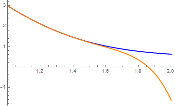
From the above graph, we see that the ADM solution ϕ5(x) is almost indistinguishable from the exact solution within the interval [1, 1.5]. However, for x ≥ 1.6, the ADM solution begins to diverge from the true solution. This is typical: the convergence rate is a function of the window of observation. If the number of terms in ADM approximation increases, the approximate solution improves at high values of x. From here, we conclude that as x increases, so does the number of ADM terms needed to obtain an accurate solution.    ■


Now we turn our attention to initial value problems for nonlinear differential equations such as

\[ \frac{{\text d}y}{{\text d}x} + a(x)\,y(x) + b(x) \, N[y] = g(x), \qquad y(x_0 ) = y_0 . \]
Here 𝑎(x), b(x), and g(x) are known and bounded functions in variable x, and N[y] is a nonlinear (analytic) operator acting on dependent variable (function) y(x) and may depend on independent variable explicitly. As before, we define the derivative operator \( \texttt{D} = {\text d}/ {\text d}x \) with respect to independent variable x and rewrite the given initial value problem in operator form:
\[ L \left[ y \right] = f \left( x, y \right) , \qquad y(x_0 ) = y_0 , \]
where the differential operator L and input function f could be chosen in different ways. Here we consider separately two options.

Option 1: \( \displaystyle L = \texttt{D} = {\text d}/ {\text d}x \) and \( \displaystyle f(x,y) = g(x) - a(x)\,y(x) - b(x)\,N[y] . \)

The main idea of the Adomian decomposition method is to represent the nonlinear term as the sum of Adomian polynomials:

\[ - a(x) - b(x)\,N[y] = \sum_{n\ge 0} A_n (u_0 , u_1 , \ldots , u_n) , \]
where An are specifically generated for each nonlinear operator according to the formula:
\[ A_n (u_0 , y_1 , \ldots , u_n) = -\left. \frac{1}{n!} \, \frac{{\text d}^n}{{\text d} \lambda^n} \left( a(x) + b(x)\, N \right) \left[ \sum_{k=0}^n u_k \lambda^k \right] \right\vert_{\lambda =0} , \qquad n=0,1,2,3,\ldots . \]
In particular,
\begin{align*} A_0 &= -a(x) - b(x)\,N[u_0 ] = f(x, u_0 ), \\ A_1 &= y_1 \,\frac{{\text d}\, f[u_0 ]}{{\text d} u_0} , \\ A_2 &= y_2 \,\frac{{\text d}\, f[u_0 ]}{{\text d} y_0} + \frac{u_1^2}{2!} \,\frac{{\text d}^2 \, f[u_0 ]}{{\text d} u_0^2} , \\ A_3 &= u_3 \,\frac{{\text d}\, f[u_0 ]}{{\text d} u_0} + u_1 u_2 \,\frac{{\text d}^2 \, N[u_0 ]}{{\text d} u_0^2} + \frac{u_1^3}{3!} \,\frac{{\text d}^3 \, N[u_0 ]}{{\text d} u_0^3} , \\ A_4 &= u_4 \,\frac{{\text d}\, f[u_0 ]}{{\text d} u_0} + \left( u_1 u_3 + \frac{u_2^2}{2!} \right) \frac{{\text d}^2 \, f[y_0 ]}{{\text d} u_0^2} + \frac{u_1^2 u_2}{2!} \,\frac{{\text d}^3 \, f[y_0 ]}{{\text d} u_0^3} + \frac{u_1^4}{4!} \,\frac{{\text d}^4 \, f[u_0 ]}{{\text d} u_0^4} , \\ A_5 &= u_5 \,\frac{{\text d}\, f[u_0 ]}{{\text d} u_0} + \left( u_1 u_4 + u_2 u_3 \right) \frac{{\text d}^2 \, N[y_0 ]}{{\text d} y_0^2} + \frac{1}{2} \left( y_1 u_2^2 + u_1^2 u_3 \right) \frac{{\text d}^3 \, f[u_0 ]}{{\text d} u_0^3} + \frac{u_1^3 u_2}{3!} \,\frac{{\text d}^4 \, f[u_0 ]}{{\text d} u_0^4} + \frac{u_1^5}{5!} \,\frac{{\text d}^5 \, f[u_0 ]}{{\text d} u_0^5} , \\ A_6 &= u_6 \,\frac{{\text d}\, f[u_0 ]}{{\text d} u_0} + \left( u_2 u_4 + \frac{u_3^2}{2!} + u_1 u_5 \right) \frac{{\text d}^2 \, f[u_0 ]}{{\text d} u_0^2} + \left( \frac{u_1^2 u_4}{2!} + \frac{u_2^3}{3!} + u_1 u_2 u_3 \right) \frac{{\text d}^3 \, f[u_0 ]}{{\text d} u_0^3} + \cdots , \end{align*}
and so on. Then we seek the solution as infinite series \( y = u_0 + u_1 + u_2 + \cdots , \) where each term un is identified by the formulae
\begin{align*} \texttt{D}\, u_0 &= f(x , u_0 ) = g(x) - a(x)\, u_0 - b(x) \,N\left[ u_0 \right] , \qquad u_0 (x_0 ) = y_0 , \\ \texttt{D}\, u_n &= A_{n-1} \left( u_0 , u_1 , \ldots , u_{n-1} \right) , \qquad u_n (0) =0 , \quad n=1,2,\ldots . \end{align*}
The right-hand side in each recursive equation is a known function in independent variable, so we can just simply integrate and find each term un explicitly:
\begin{align*} u_0 (x) &= y_0 + \int_{x_0}^x \, f(t , y_0 )\,{\text d}t , \\ u_n (x) &= \int_{x_0}^x A_{n-1} \left( u_0 , u_1 , \ldots , u_{n-1} \right) {\text d}x , \qquad n=1,2,\ldots . \end{align*}

Option 2: \( \displaystyle L = \texttt{D} + a(x) \) and \( \displaystyle f(x,y) = g(x) - b(x)\,N[y] . \)

In this case, one have to solve a linear differential equation \( L\left[ y \right] = \varphi (x) \) at each step for some known function φ:
\[ L^{-1} \left[ y \right] (x) = y (x_0 ) + \mu^{-1} (x) \int_{x_0}^x \varphi (s)\,\mu (s) \,{\text d} s , \qquad \mbox{where } \mu (x) = \exp \left\{ \int a(x)\,{\text d} x \right\} . \]
The required solution of the given initial value problem has the same form
\[ y(x) = u_0 (x) + u_1 (x) + u_2 (x) + \cdots , \]
where each term is determined recursively: \begin{align*} \texttt{D}\, u_0 + a(x)\, u_0 (x) &= f(x , y_0 ) = g(x) - b(x)\,N \left[ y_0 \right] , \qquad u_0 (0) = y_0 , \\ \texttt{D}\, u_n + a(x)\, u_n (x) &= A_{n-1} \left( u_0 , u_1 , \ldots , u_{n-1} \right) , \qquad u_n (0) =0 , \quad n=1,2,\ldots . \end{align*}
The Adomian polynomials in our case correspond to the function \( f(x) = g(x) - b(x)\,N[y] . \)    ▣

Example: We apply the Adomian decomposition method to find an approximate solution to the initial value problem for logistic equation:

\[ \dot{P} = 0.02\,P(1-P) , \qquad P(0) = P_0 = 10. \]
This problem has a unique solution
\[ P(t) = \frac{10\, e^{t/50}}{10\, e^{t/50} -9} , \qquad t\ge 0, \]
as Mathematica confirms
DSolve[{P'[t] == 2/100*P[t]*(1 - P[t]), P[0] == 10}, P[t], t]
We expand the nonlinear term N[P] = P2 into the series:
\[ N[P] = P^2 = \sum_{n\ge 0} A_n (P_0 , P_1 , \ldots P_n ) , \]
where first five polynomials are not hard to determine manually:
\begin{align*} A_0 &= y_0^2 = 10^2 = 100, \\ A_1 &= y_1 \,2\, y_0 , \\ A_2 &= y_2 \,2\, y_0 + y_1^2 , \\ A_3 &= y_3 \,2\, y_0 + 2\,y_1 y_2 , \\ A_4 &= y_4 \,2\, y_0 + 2\, y_1 y_3 + y_2^2 , \\ A_5 &= y_5 \,2\, y_0 + 2\,y_1 y_4 + 2\,y_2 y_3 . \end{align*}
Substituting expansion \( P = u_0 + u_1 + u_2 + \cdots \) into the given logistic equation, we get
\[ \texttt{D} \left( u_0 + u_1 + u_2 + \cdots \right) = 0.02 \left( u_0 + u_1 + u_2 + \cdots \right) - 0.02 \left( A_0 + A_1 + A_2 + \cdots \right) . \]
For the first term, we have the initial value problem
\[ \texttt{D} \, u_0 = 0, \qquad u_0 (0) = 10 . \]
Solving the initial value problem for the above linear equation we get the first term:
\[ u_0 (t) = 10 . \]
For the next terms, we have
\[ \texttt{D} \, u_n \equiv \dot{u}_n = 0.02 \, u_{n-1} - 0.02\,A_{n-1} , \qquad u_n (0) = 0 , \quad n=1,2,3,\ldots ; \]
which is a linear differential equation with respect to un. Solving these equations recursively, we obtain
\begin{align*} u_1 &= -\frac{9}{5}\,t , \qquad &A_1 = -36\,t , \\ u_2 &= \frac{171}{500} \,t^2 , \qquad &A_2 = \frac{252}{25}\,t^2 , \\ u_3 &= -\frac{1623}{25000} \,t^3 , \qquad &A_3 = -\frac{1581}{625} \, t^3 , \\ u_4 &= \frac{61617}{5000000} \,t^4 , \qquad &A_4 = \frac{74643}{125000} \, t^4 , \\ u_5 &= -\frac{2924103}{1250000000} \, t^5 , \qquad &A_5 = - \frac{4236099}{31250000} \, t^5 . \end{align*}
u[0, t] := 10
A[0, t] := 100
u[1, t_] = f[t] /. First@ DSolve[{f'[t] == (1/50)*u[0,t] - (1/50)*100, f[0] == 0}, f, t]
A[1, t] = -2*u[0,t]*u[1,t]
u[2, t_] = f[t] /. First@ DSolve[{f'[t] == (1/50)*u[1, t] - (1/50)*A[1, t], f[0] == 0}, f, t]
A[2,t_]=20*u[2,t] + (u[1,t])^2
u[3, t_] = f[t] /. First@ DSolve[{f'[t] == (1/50)*u[2, t] - (1/50)*A[2, t], f[0] == 0}, f, t]
A[3,t_]= 20*u[3,t] + 2*u[1,t]*u[2,t]
u[4, t_] = f[t] /. First@ DSolve[{f'[t] == (1/50)*u[3, t] - (1/50)*A[3, t], f[0] == 0}, f, t]
A[4,t_]= 20*u[4,t] + (u[2,t])^2 + 2*u[1,t]*u[3,t]
u[5, t_] = f[t] /. First@ DSolve[{f'[t] == (1/50)*u[4, t] - (1/50)*A[4, t], f[0] == 0}, f, t]
Then we plot the exact solution in blue and ADM approximation in orange:
z[t_] = 10*Exp[t/50]/(10*Exp[t/50] - 9)
phi[t_] := 10 - (9 t)/5 + (171 t^2)/500 - (1623 t^3)/25000 + (61617 t^4)/ 5000000 - (2924103 t^5)/1250000000
Plot[{z[t], phi[t]}, {t, 0, 3.0}, PlotStyle -> {{Thick, Blue}, {Thick, Orange}}]
A[5, t_] = -4236099*t^5 /1250000000;
u[6, t_] = f[t] /. First@ DSolve[{f'[t] == (1/50)*u[5, t] - (1/50)*A[5, t], f[0] == 0}, f, t]
phi6[t] = phi[t] - u[6, t]
Plot[{z[t], phi[t], phi6[t]}, {t, 0, 8}, PlotStyle -> {{Thick, Blue}, {Thick, Orange}, {Thick, Magenta}}]
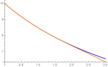
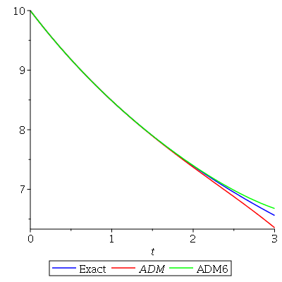
As we see, the ADM approximation with six terms (green) is more accurate to the actual solution (in blue) than the ADM approximation with five terms (in red).

Let us compare the obtained Adomian approximation with the true solution:

\[ P(t) = \frac{10\, e^{t/50}}{10\, e^{t/50} -9} = 10 - \frac{9\,t}{5} + \frac{171}{500}\,t^2 - \frac{1623}{25000}\,t^3 + \frac{61617}{5000000}\, t^4 + \cdots . \]
according to Mathematica:
Series[10*Exp[t/50]/(10*Exp[t/50]-9), {t,0,7}]
10 -
Therefore, we confirm that the Adomian method provides the true solution.

Finally, we apply the Adomian's decomposition method with accelerated polynomials to this initial value problem. We proceed exactly in the same manner as the ADM requires, but use accelerated polynomials aAn instead of the classical Adomian polynomials An. We start with

\[ aA_0 = N\left[ u_0 \right] = N\left[ 10 \right] = -0.02\left( 1- -10^2 \right) = -1.8 = -\frac{9}{5} , \]
because \( N\left[ y \right] = 0.02\left( y - y^2 \right) . \) The first term is obtained by solving the initial value problem:
\[ \dot{u}_1 = aA_0 = -1.8, \qquad u_1 (0) =0 . \]
This gives \( u_1 (t) = -9\,t/5 . \) Then we calculate the second term
\begin{align*} aA_1 &= N \left[ u_0 + u_1 \right] - N \left[ u_0 \right] = 0.02 \, N\left[ 10 - \frac{9}{5}\,t \right] - o.02\, N\left[ 10 \right] = -\frac{9t\left( 9t -95 \right)}{1250} , \\ u_2 (t) &= - \frac{9}{2500} \left( 6\,t^3 -95\,t^2 \right) , \end{align*}
because
DSolve[{u'[t]==-9*t*(9*t-95)/1250 , u[0]==0}, u[t],t]
u[t]
The next accelerated polynomial becomes
\begin{align*} aA_2 &= N \left[ u_0 + u_1 + u_2 \right] - N \left[ u_0 + u_1 \right] \\ &= 0.02 \left( u_0 + u_1 \right)^2 -0.02 \left( u_0 + u_1 + u_2 \right)^2 \\ &= -0.02 \,u_2 \left( u_2 + 2\,u_1 + 2\,u_0 \right) \end{align*}
   ■

Example: Consider the initial value problem for the logistic equation

\[ \frac{{\text d}P}{{\text d}t} = P(t) \left( 1- P \right) + e^{-2t} , \qquad P(0) = 2 . \]
This problem has the solution:
\[ P(t) = 1 + \sqrt{e^{-2t}} \]
because
DSolve[{y'[t] == y[t]*(1 - y[t]) + Exp[-2*t], y[0] == 2}, y[t], t]
{{y[t] -> 1 + Sqrt[E^(-2 t)]}}
Its power series solution is
\[ P(t) = 2 -t + \frac{t^2}{2} - \frac{t^3}{6} + \frac{t^4}{24} - \frac{t^5}{120} + \frac{t^6}{720} - \frac{t^7}{5040} + \frac{t^8}{40320} - \frac{t^9}{362880} + \frac{t^{10}}{3628800} + \cdots . \]
because
Series[1 + Sqrt[E^(-2 t)], {t, 0, 10}]
\( \displaystyle 2 -t + \frac{t^2}{2} - \frac{t^3}{6} + \frac{t^4}{24} - \frac{t^5}{120} + \frac{t^6}{720} - \frac{t^7}{5040} + \frac{t^8}{40320} - \frac{t^9}{362880} + \frac{t^{10}}{3628800} + O[t]^{11} \)
We expand the nonhomogeneous term
\[ e^{-2t} = \sum_{n\ge 0} (-2)^n \frac{t^n}{n!} . \]
Note also that the first few Adomian polynomials for the nonlinear term P²(t) are given by:
\begin{eqnarray*} A_0 &=& - u_0^2 = - 4, \\ A_1 &=& -2 u_0 u_1 = -4\,u_1 , \\ A_2 &=& - u_1^2 -2\,u_0 u_2 , \\ A_3 &=& -2\,u_0 u_3 -2\,u_1 u_2 , \\ A_4 &=& -2\,u_0 u_4 -u_2^2 -2\,u_1 u_3 , \end{eqnarray*}
and so on. Representing the solution as infinite series, we have \( P(t) = \sum_{n\ge 0} u_n (t) , \) where u0 = 2. Applying the recursion scheme
\[ \dot{u}_{n+1} = \left( -2 \right)^n \frac{t^n}{n!} + u_n (t) + A_n (t) , \qquad u_{n+1} (0) =0, \]
gives:
\begin{eqnarray*} u_1 &=& t + \int_0^t A_0 \,{\text d}x + \int_0^t u_0 \,{\text d}x = t \left( 1 -4 + 2 \right) = -t . \\ u_2 &=& -t^2 + \int_0^t A_1 (x) \,{\text d}x + \int_0^t u_1 (x) \,{\text d}x = t^2 \left( -1 + \frac{4}{2} - \frac{1}{2} \right) = \frac{t^2}{2} , \\ u_3 &=& 2\,\frac{t^3}{3} + \int_0^t A_2 \,{\text d}x + \int_0^t u_2 \,{\text d}x = - \frac{t^3}{6} , \\ u_4 &=& - 2^3 \frac{t^4}{24} + \int_0^t A_3 \,{\text d}x + \int_0^t u_3 = - 2^3 \frac{t^4}{24} + \frac{10}{24}\,t^4 - \frac{t^4}{24} = \frac{t^4}{24} , \end{eqnarray*}
and so on. Upon adding all these terms, we obtain a truncated power series of a true solution.    ■

Example: Consider the initial value problem for the integro-differential equation

\[ \dot{y} = 2.3\, y -0.01\,y^2 -0.1\,y\, \int_0^t y(\tau )\,{\text d}\tau , \qquad y(0) =50. \]
Using ADM method, we seek an approximate solution in the form
\[ y = u_0 + u_1 + u_2 + \cdots , \]
where \( u_0 =50 \) and nonlinear operator N[y] is expanded into Adomian polynomials:
\[ N[y] \equiv -0.01\,y^2 -0.1\,y\, \int_0^t y(\tau )\,{\text d}\tau = A_0 + A_1 + A_3 + \cdots . \]
Since
\[ \frac{{\text d}\, N[y ]}{{\text d} y} = -0.02\,y - 0.1\,y^2 - 0.1\,\int_0^t y(\tau )\,{\text d}\tau , \quad \frac{{\text d}^2\, N[y ]}{{\text d} y^2} = -0.02 -0.3\,y , \quad \frac{{\text d}^3\, N[y ]}{{\text d} y^3} = -0.3 , \quad \frac{{\text d}^k\, N[y ]}{{\text d} y^k} = 0, \quad k= 4,5 , \ldots , \]
we have
\begin{align*} A_0 &= -0.01\,50^2 - 0.1\,50\, \int_0^t 50\,{\text d}\tau = -25 -250\,t , \\ A_1 &= -u_1 \left( 1+ 5t \right) - 5\,\int_0^t u_1 (\tau ) \,{\text d}\tau , \\ A_2 &= -u_2 \left( 1+ 5t \right) - \frac{u_1^2}{100} - \frac{u_1}{10} \, \int_0^t u_1 (\tau ) \,{\text d}\tau -5 \int_0^t u_2 (\tau ) \,{\text d}\tau , \\ A_3 &= - u_3 \left( 1+ 50t \right) -\frac{1}{50}\,u_1 u_2 - \frac{u_2}{10} \, \int_0^t u_1 (\tau ) \,{\text d}\tau - \frac{u_1}{10} \, \int_0^t u_2 (\tau ) \,{\text d}\tau - 50 \int_0^t u_3 (\tau ) \,{\text d}\tau , \\ A_4 &= -u_4 \left( 1+ 5t \right) -\frac{1}{100}\,u_2^2 - \frac{1}{50}\,u_1 u_3 - \frac{u_3}{10} \, \int_0^t u_1 (\tau ) \,{\text d}\tau - \frac{u_2}{10} \, \int_0^t u_2 (\tau ) \,{\text d}\tau - \frac{u_1}{10} \, \int_0^t u_3 (\tau ) \,{\text d}\tau -5 \int_0^t u_4 (\tau ) \,{\text d}\tau , \\ A_5 &= - u_5 \left( 1+ 50t \right) -\frac{1}{50}\,u_2 u_3 -\frac{1}{50}\,u_1 u_4 - \frac{u_4}{10} \, \int_0^t u_1 (\tau ) \,{\text d}\tau - \frac{u_3}{10} \, \int_0^t u_2 (\tau ) \,{\text d}\tau - \frac{u_2}{10} \, \int_0^t u_3 (\tau ) \,{\text d}\tau - \frac{u_1}{10} \, \int_0^t u_4 (\tau ) \,{\text d}\tau -50 \int_0^t u_5 (\tau ) \,{\text d}\tau . \end{align*}
Now we are ready to construct 6-term ADM approximation
\[ {\texttt D} u_n = 2.3\,u_{n-1} + A_{n-1}, \quad u_n (0) =0, \qquad n=1,2,3,\ldots . \]
Using Mathematica, we perform every step explicitly (without automatic looping).
u[0, t_] := 50
A[0, t_] = -1/100*50^2 - 1/10*50*Integrate[50, {x, 0, t}]
u[1, t_] = f[t] /. First@ DSolve[{f'[t] == 23*5 + A[0, t], f[0] == 0}, f, t]
Out[20]= -25 - 250 t
Out[21]= -5 (-18 t + 25 t^2)
For the second stage, we get
A[1, t_] = -Simplify[u[1, t]*(1 + 5*t) + 5*Integrate[u[1,x], {x, 0, t}]]
u[2, t_] = f[t] /. First@ DSolve[{f'[t] == 23*u[1,t]/10 + A[1, t], f[0] == 0}, f, t]
Out[22]= -(10/3) t (27 + 165 t - 250 t^2)
Out[23]= 1/6 (351 t^2 - 1675 t^3 + 1250 t^4)
A[2, t_] = -Simplify[u[2, t]*(1 + 5*t) + (u[1,t])^2 /100 + 5*Integrate[u[2,x], {x, 0, t}] + u[1,t]*Integrate[u[1,x], {x, 0, t}]/10]
u[3, t_] = f[t] /. First@ DSolve[{f'[t] == 23*u[2,t]/10 + A[2, t], f[0] == 0}, f, t]
Out[24]= -(1/24) t^2 (3348 + 6980 t - 55625 t^2 + 42500 t^3)
Out[25]= 1/720 (-1188 t^3 - 167925 t^4 + 402750 t^5 - 212500 t^6)
Then on the third stage, we have
A[3, t_] = -Simplify[u[3, t]*(1 + 50*t) + u[1, t]*u[2, t]/50 + u[2,t]*Integrate[u[1,x], {x, 0, t}]/10 + u[1,t]*Integrate[u[2,x], {x, 0, t}]/10 + 50 *Integrate[u[3,x], {x, 0, t}] ]
u[4, t_] = f[t] /. First@ DSolve[{f'[t] == 23*u[3, t]/10 + A[3, t], f[0] == 0}, f, t]
Out[26]= (t^3 (-522396 + 2753625 t + 74256000 t^2 - 177218125 t^3 + 92000000 t^4))/5040
Out[27]= (-1353807 t^4 + 100065 t^5 + 134567125 t^6 - 258056250 t^7 + 115000000 t^8)/50400
Finally, we obtain
A[4, t_] = -Simplify[u[4, t]*(1 + 5*t) + (u[2,t])^2 /100 + u[3,t]*u[1,t]/50 + u[3,t]*Integrate[u[1,x], {x, 0, t}]/10 + u[2,t]*Integrate[u[2,x], {x, 0, t}]/10 + u[1,t]*Integrate[u[3,x], {x, 0, t}]/10 + 5*Integrate[u[4,x], {x, 0, t}] ]
u[5, t_] = f[t] /. First@ DSolve[{f'[t] == 23*u[4, t]/10 + A[4, t], f[0] == 0}, f, t]
Out[28]= -((t^4 (7967484 - 1448901972 t + 5233879350 t^2 + 26405797500 t^3 - 60180328125 t^4 + 27762500000 t^5))/1814400)
Out[29]= (1/45360000)(-600313518 t^5 + 6071613975 t^6 + 21100995000 t^7 - 149290171875 t^8 + 193617578125 t^9 - 69406250000 t^10)
Now we add these five terms and plot two ADM approximations
phi5[t_] = u[0, t]
Do[phi5[t] = phi5[t] + u[j, t], {j, 1, 5}]
A[5, t_] = -Simplify[ u[5, t]*(1 + 50*t) + u[2, t]*u[3, t]/50 + u[4, t]*u[1, t]/50 + u[4, t]*Integrate[u[1, x], {x, 0, t}]/10 + u[3, t]*Integrate[u[2, x], {x, 0, t}]/10 + u[2, t]*Integrate[u[3, x], {x, 0, t}]/10 + u[1, t]*Integrate[u[4, x], {x, 0, t}]/10 + 50*Integrate[u[5, x], {x, 0, t}]]
u[6, t_] = f[t] /. First@ DSolve[{f'[t] == 23*u[5, t]/10 + A[5, t], f[0] == 0}, f, t]
phi6[t_] = phi5[t]+u[6,t]
Plot[Tooltip@{phi5[t], phi6[t]}, {t, 0, 0.8}, PlotStyle -> {Red, Green}, PlotLegends -> {"ADM(5)", "ADM(6)"}]
   ■


In all problems, y' denotes the derivative of function y(x) with respect to independent variable x and \( \dot{y} = {\text d} y/{\text d}t \) denotes the derivative with respect to time variable.
  1. Using ADM, solve the initial value problem: \( y' + \sqrt{y} = 2x , \quad y(0) =1 . \)
  2. Using ADM, solve the initial value problem: \( y' + \sqrt{y} = 1+x+x^2 , \quad y(0) =2 . \)
  3. Using ADM, solve the initial value problem: \( y' + \sqrt{1+y} = 0 , \quad y(0) =3 . \)
  4. Using ADM, solve the initial value problem: \( y' + 2x\, y = 1+ x^2 + y^2 , \quad y(0) =1 . \)
  5. Using ADM, solve the initial value problem: \( y' + 2x\, y = e^x + 2y\left( \ln y \right)^2 , \quad y(0) =1 . \)
  6. Using ADM, solve the initial value problem: \( y' = y^p , \quad y(0) =1 ; \) with p ≥ 1.

    Its true solution is

    \[ y^{-1} (t) = \left( 1 - (p-1)t \right)^{1/(p-1)} \]
  7. Using ADM, solve the initial value problem: \( y' = 2y - y^2 , \quad y(0) =1 . \)

    Its true solution is y(t) = 1 + tanh(t)

  8. Using ADM, solve the initial value problem: \( y' = x+ e^{-y} , \quad y(0) =0 . \)

    Its true solution is \( y(x) = \frac{x^2}{2} + \ln \left( 1 +\sqrt{\frac{\pi}{2}}\,\mbox{erf} \left( \frac{x}{\sqrt{x}} \right) \right) \) for x > -1.2755, where erf(x) = \( \frac{2}{\sqrt{\pi}} \int_0^x e^{-t^2}\,{\text d}t . \)

Complete List of Publications using Adomian Decomposition Method

  1. Duan, J.-S., Convenient analytic recurrence algorithms for the Adomian polynomials, Applied Mathematics and Computation, 2011, Vol. 217, No. 13, pp. 6337--6348.
  2. Duan, J.-S., New recurrence algorithms for the nonclassic Adomian polynomials, Computers and Mathematics with Applications, 2011, Vol. 62 No. 8, pp. 2961--2977.
  3. Duan, J.-S. and Guo, A.-P., Reduced polynomials and their generation in Adomian decomposition methods, CMES: Computer Modeling in Engineering and Sciences, 2010, Vol. 60, No. 2, pp. 139--150.
  4. Duan, J.-S. and Guo, A.-P., Symbolic implementation of a new, fast algorithm for the multivariable Adomian polynomials, Proceedings of the 2011 World Congress on Engineering and Technology (CET 2011), Shanghai, China, October 28 - November 2, 2011, Vol. 1, IEEE Press, Beijing, pp. 72--74.
  5. Duan, J.-S. and Rach, R., New higher-order numerical one-step methods based on the Adomian and the modified decomposition methods, Applied Mathematics and Computation, 2011, Vol. 218 No. 6, pp. 2810-2828.
  6. Duan, J.-S. and Rach, R., The degenerate form of the Adomian polynomials in the power series method for nonlinear ordinary differential equations, Journal of Mathematics and System Science, Volume 5, Pages 411--428, 2015.
  7. Duan, J.-S., Rach, R., Baleanu, D., and Wazwaz, A.-M., A review of the Adomian decomposition method and its applications to fractional differential equations Communications in Fractional Calculus, Volume 3, Issue 2, 2012, Pages 73--99.
  8. Duan, J.-S. and Rach, R., Higher-order numeric Wazwaz--El-Sayed modified Adomian decomposition algorithms, Computers and Mathematics with Applications, 2012, Vol. 63 No. 11, pp. 1557--1568.
  9. Duan, J.-S., Rach, R. and Wazwaz, A.-M., Solution of the model of beam-type micro- and nano-scale electrostatic actuators by a new modified Adomian decomposition method for nonlinear boundary value problems, International Journal of Non-Linear Mechanics, 2013, Vol. 49, 159--169.
  10. J.-S. Duan, R. Rach, and A.-M. Wazwaz, A new modified Adomian decomposition method for higher-order nonlinear dynamical systems, CMES: Computer Modeling in Engineering & Sciences, 2013, Vol. 94, No. 1, pp. 77--118.
  11. J.-S. Duan, R. Rach, A.-M. Wazwaz, Temuer Chaolu, and Z. Wang, A new modified Adomian decomposition method and its multistage form for solving nonlinear boundary value problems with Robin boundary conditions, Applied Mathematical Modelling, 2013, Vol. 37, Nos. 20/21, Pages 8687--8708.
  12. A.-M. Wazwaz, R. Rach, and J.-S. Duan, Adomian decomposition method for solving the Volterra integral form of the Lane-Emden equations with initial values and boundary conditions, Applied Mathematics and Computation, 2013, Volume 219, Issue 10, Pages 5004--5019; doi: 10.1016/j.amc.2012.11.012
  13. R. Rach, A.-M. Wazwaz, and J.-S. Duan, A reliable modification of the Adomian decomposition method for higher-order nonlinear differential equations, Kybernetes, 2013, Volume 42, Issues 1/2, Pages 282--308
  14. Jun-Sheng Duan, Zhong Wang, Shou-Zhong Fu, and Temuer Chaolu, Parameterized temperature distribution and efficiency of convective straight fins with temperature-dependent thermal conductivity by a new modified decomposition method, International Journal of Heat and Mass Transfer, Vol. 59 (2013) 137--143.
  15. A.-M. Wazwaz, R. Rach, L. Bougoffa, and J.-S. Duan, Solving the Lane-Emden-Fowler type equations of higher orders by the Adomian decomposition method, CMES: Computer Modeling in Engineering & Sciences, Vol. 100, No. 6, pp. 507--529, 2014, doi:10.3970/cmes.2014.100.507.
  16. J.-S. Duan, R. Rach, and A.-M. Wazwaz, A reliable algorithm for positive solutions of nonlinear boundary value problems by the multistage Adomian decomposition method, Open Engineering, Volume 5, Issue 1, 59--74, 2014. doi: 10.1515/eng-2015-0007
  17. R. Rach, A.-M. Wazwaz, and J.-S. Duan, A reliable analysis of oxygen diffusion in a spherical cell with nonlinear oxygen uptake kinetics, International Journal of Biomathematics, Vol. 07, No. 02, March 2014, 1450020 (2014) [12 pages] doi: 10.1142/S179352451450020X.
  18. Rach, R. Duan,J.-S., and Wazwaz, A.-M., Solving coupled Lane-Emden boundary value problems in catalytic diffusion reactions by the Adomian decomposition method Journal of Mathematical Chemistry, Volume 52, Issue 1, 2014, Pages 255--267.
  19. Wazwaz, A.-M., Rach, R., and Duan, J.-S., A study on the systems of the Volterra integral forms of the Lane-Emden equations by the Adomian decomposition method, Mathematical Methods in the Applied Sciences, Vol. 37, Issue 1, 2014, Pages 10--19.
  20. R. Rach, J.-S. Duan, and A.-M. Wazwaz, On the solution of non-isothermal reaction-diffusion model equations in a spherical catalyst by the modified Adomian method, Chemical Engineering Communications, Volume 202, Issue 8, 2015, Pages 1081--1088.
  21. J.-S. Duan, R. Rach, and A.-M. Wazwaz, Oxygen and carbon substrate concentrations in microbial floc particles by the Adomian decomposition method, MATCH Communications in Mathematical and in Computer Chemistry, Vol. 73, No. 3, 2015, pp. 785--796.
  22. J.-S. Duan, R. Rach, and A.-M. Wazwaz, Steady-state concentrations of carbon dioxide absorbed into phenyl glycidyl ether solutions by the Adomian decomposition method, Journal of Mathematical Chemistry, Vol. 53, 2015, Pages 1054-1067.
  23. R. Rach, A.M. Wazwaz, and J.S. Duan, The Volterra integral form of the Lane-Emden equation: New derivations and solution by the Adomian decomposition method, Journal of Applied Mathematics and Computing, Volume 47, Issue 1, 2015, Pages 365--379.
  24. J.-S. Duan, R. Rach, and A.-M. Wazwaz, Higher-order numeric solutions of the Lane-Emden type equations derived from the multi-stage modified decomposition method, International Journal of Computer Mathematics, International Journal of Computer Mathematics, Volume 94, No. 1, 2017, 197--215.
  1. Abassy, T.A., Improved Adomian decomposition method, Computers and Mathematics with Applications, 2010, Vol.59, pp. 42--54.
  2. Daftardar-Gejji, V. and Jafari, H., An iterative method for solving nonlinear functional equations, Journal of Mathematical Analysis and Applications, 2006, Vol. 316, No. 2, pp. 753--763. https://doi.org/10.1016/j.jmaa.2005.05.009
  3. Rach, R., On the Adomian (decomposition) method and comparisons with Picard's method, Journal of Mathematical Analysis and Applications, 1987, Vol. 128, Issue 2, pp. 480--483.
  4. Rach, R., A convenient computational form for the Adomian polynomials, Journal of Mathematical Analysis and Applications, 1984, Volume 102, Issue 2, pages 415--419. https://doi.org/10.1016/0022-247X(84)90181-1
  5. Rach, R., “A new definition of the Adomian polynomials”, Kybernetes, Volume 37, Issue 7, 2008, Pages 910-955.
  6. Sari, M.R., Kezzar, M., Adjabi, R., A comparison of Adomian and generalized Adomian methods in solving the nonlinear problem of flow in convergent-divergent channels, Applied Mathematical Sciences, 2014, Vol. 8, no. 7, 321 - 336; http://dx.doi.org/10.12988/ams.2014.39495
  1. Abdelrazec, Ahmed H.M., Adomian decomposition method: convergence analysis and numerical approximations, Thesis, McMaster University, Ontario, Canada, 2008.
  2. Abdelrazec, A., and Pelinovsky, D., Convergence of the Adomian decomposition method for initial-value problems, Numerical Methods for Partial Differential Equations, 2011, Vol. 27, No. 4, 749--766, 2011. https://doi.org/10.1002/num.20549
  3. Abushammala, Mariam B.H., Iterative methods for the numerical solutions of boundary value problems, Thesis of the American University of Sharjah College of Arts and Sciences, Sharjah United Arab Emirates, June 2014.
  4. Golberg, M.A., "A note on the decomposition method for operator equation," Applied Mathematics and Computation, 1999, 106, 215--220.
  5. Himoun, N., Abbaoui, K. and Cherruault, Y. (1999), “New results of convergence of Adomian’s method”, Kybernetes, Vol. 28 No. 4, pp. 423-9.
  6. Jiao, Y.-C., Dang, C., Yamamoto, Y., An extension of the decomposition method for solving nonlinear equations and its convergence, Computers and Mathematics with Applications, 2008, Vol. 55, pp. 760--775
  7. Ray, S.S., New Approach for General Convergence of the Adomian Decomposition Method, World Applied Sciences Journal, 2014, Vol. 32, No. 11, pp. 2264--2268; doi: 10.5829/idosi.wasj.2014.32.11.1317
  8. Sunday, J., Convergence analysis and implementation of Adomian decomposition method on second-order oscillatory problems, Asian Research Journal of Mathematics, 2017, Vol. 2, No. 5, pp. 1--12. Article no.ARJOM.32011


Return to Mathematica page
Return to the main page (APMA0330)
Return to the Part 1 (Plotting)
Return to the Part 2 (First Order ODEs)
Return to the Part 3 (Numerical Methods)
Return to the Part 4 (Second and Higher Order ODEs)
Return to the Part 5 (Series and Recurrences)
Return to the Part 6 (Laplace Transform)
Return to the Part 7 (Boundary Value Problems)