Return to computing page for the second course APMA0340
Return to computing page for the fourth course APMA0360
Return to Mathematica tutorial for the first course APMA0330
Return to Mathematica tutorial for the second course APMA0340
Return to Mathematica tutorial for the fourth course APMA0360
Return to the main page for the course APMA0330
Return to the main page for the course APMA0340
Return to the main page for the course APMA0360
Return to Part I of the course APMA0330
Glossary
Plotting Solutions of ODEs
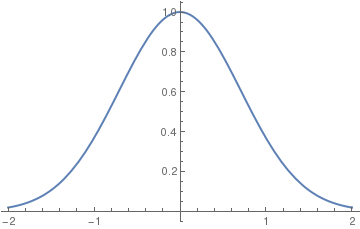
When Mathematica is capable to find a solution (in explicit or implicit form) to an initial value problem, it can be plotted as follows. Let us consider the initial value problem
Plot[y[x] /.a, {x,-2,2}, PlotStyle -> Thick]
In this command sequence, I am first defining the differential equation that I want to solve. In this line, I define the equation
and the initial condition as well as the independent and dependent variables.
In the second line, I am commanding Mathematica to evaluate the given differential equation and plot its result. I then
command Mathematica to solve the equation and plot the given result of the initial value problem for the range listed above.
Typing these two commands together allows Mathematica to solve the initial value problem for you and to graph the initial
value problem's solution.
 |
Another option:
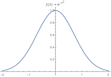
a = DSolve[{y'[x] == -2 x y[x], y[0] == 1}, y[x], x];
Trace[DSolve[{y'[x] == -2 x y[x], y[0] == 1}, y[x], x]] Plot[y[x] /. a, {x, -2, 2}, PlotStyle -> Thick, PlotLabel -> a[[1, 1]]] |
|
| Solution to the IVP. | Mathematica code |
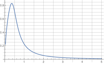
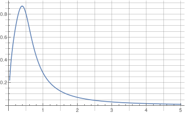
If you need to plot a sequence of solutions with different initial conditions, one can use the following script:
IC = {{0.5, 0.7}, {0.5,(*4*).8}, {0.5, 1}};
Do[ansODE[i] = Flatten[DSolve[{myODE, y[IC[[i, 1]]] == IC[[i, 2]]}, y[t], t]]; myplot[i] = Plot[Evaluate[y[t] /. ansODE[i]], {t, 0.02, 5}, GridLines -> All, PlotRange -> All, PlotStyle -> Thick];
Print[myplot[i]];, {i, 1, Length[IC]}]
DSolve::bvnul: For some branches of the general solution, the given boundary conditions lead to an empty solution. >>
DSolve::bvnul: For some branches of the general solution, the given boundary conditions lead to an empty solution. >>
DSolve::bvnul: For some branches of the
general solution, the given
boundary conditions lead to an empty solution. >>
General::stop: Further output of DSolve::bvnul will be suppressed
during this calculation. >>
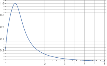
In the above script, you define the differential equation that you want to solve and the initial conditions (the respective x and y values). Flattening creates a list of the equations. Then you are asking Mathematica to evaluate the different equations according to their different initial conditions.
Finally, the Print command tells Mathematica to plot the graphs and the size that you want the lines on the graphs to be.
When you enter these commands, you may receive a line saying that some of the branches lead to empty solutions, but this just means that DSolve cannot find a unique solution for part of the equation. However, this does not appear to affect the final graph.
To plot a family of solutions to Clairaut's equation, we type:
samples1 = Table[f1[x], {c, -20/3, 8, 1}]
Plot[Evaluate[samples1], {x, -3, 3}, PlotStyle -> {Black}]
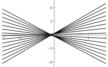
In this command, I am plotting a family of solutions to a differential equation. This command is not really any different from a normal plot command. The primary difference is that I have created a list of samples in a table. These samples have the variable c and then I can plug in different values of c to create the values in this table. This means that I am asking Mathematica to plot solutions with different values of the differential constant c. This command will plot a variety of different graphs over the range of c. The command on the second line also yields the different members of this family of equations associated with each value of c.
Plot[y'[x] = -Sqrt[a^2 - x^2]/x, {x, 0, 20},
PlotRange -> {-10, 10}], {a, 0, 20}]
a Log[x] + a Log[a^2 + a Sqrt[a^2 - x^2]]]}}
Plot[-Sqrt[a^2 - x^2] + a Log[a] - a Log[a^2] - a Log[x] + a Log[a^2 + a Sqrt[a^2 - x^2]], {x, 0, 20}, PlotRange -> All], {a, 1, 20}]
Now suppose we want to plot solutions to Riccati differential equation subject to different initial conditions:
parSol = Quiet[ ParametricNDSolve[{y'[x] == x^2 - (y[x])^2, y[0] == y0}, y, {x, -2, 10}, {y0}, WorkingPrecision -> 22]];
vals = {1, 2, 0, -.3, -.5, -.6, -1}
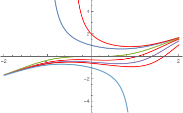
You still can use NDSolve, but for a single eigenvalue:
p1 = Plot[Evaluate[y[x] /. s1], {x, -2, 10}, PlotStyle -> {Thick, Purple}, PlotRange -> {-5, 5}]
Return to Mathematica page
Return to the main page (APMA0330)
Return to the Part 1 (Plotting)
Return to the Part 2 (First Order ODEs)
Return to the Part 3 (Numerical Methods)
Return to the Part 4 (Second and Higher Order ODEs)
Return to the Part 5 (Series and Recurrences)
Return to the Part 6 (Laplace Transform)
Return to the Part 7 (Boundary Value Problems)