Return to computing page for the second course APMA0340
Return to Mathematica tutorial for the first course APMA0330
Return to Mathematica tutorial for the second course APMA0340
Return to the main page for the course APMA0330
Return to the main page for the course APMA0340
Return to Part IV of the course APMA0330
Glossary
Applications
We present some applications of differential equations of order greater than one.
Example: (Flow Problem) A 500 liter container initially contains 10 kg of salt. A brine mixture of 100 grams of salt per liter is entering the container at 6 liter per minute. The well-mixed contents are being discharged from the tank at the rate of 6 liters per minute.
Express the amount of salt in the container as a function of time.
Salt is coming at the rate: 6*(0.1)=0.6 kg/min
d yin /dt =0.6 ; d yout/dt = 6x/500
dx/dt = 0.6 -6x/500 ; x(0)=10
Suppose that the rate of discharge is reduced to 5 liters per minute.
SolRule[t_] = Apart[x[t] /. First[%]]
Together[SolRule'[t] == Together[6/10 - 5*SolRule[t]/(500 + t)]]
SolRule[0]
Out[4]= True
Out[5]= 10
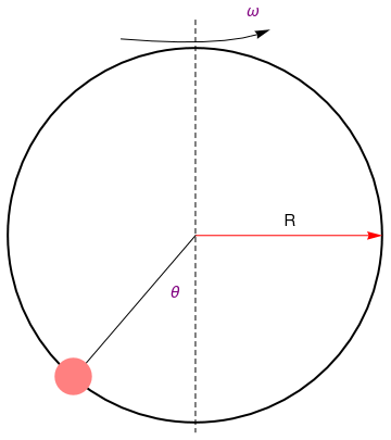
Example: Consider a bead of mass m on a rotating hoop of radius R.
disk = Graphics[{Pink, Disk[{-0.65, -0.75}, 0.1]}]
linev = Graphics[{Dashed, Line[{{0, 1.15}, {0, -1.05}}]}]
line = Graphics[Line[{{0, 0}, {-0.6, -0.7}}]]
ar = Graphics[ Arrow[BezierCurve[{{-0.4, 1.05}, {0.2, 1}, {0.4, 1.1}}]]]
arrow = Graphics[{Red, Arrow[{{0, 0}, {1, 0}}]}]
text1 = Graphics[ Text[Style["\[Theta]", FontSize -> 14, Purple], {-0.11, -0.3}]]
text2 = Graphics[ Text[Style["\[Omega]", FontSize -> 14, Purple], {0.31, 1.2}]]
text3 = Graphics[Text[Style["R", FontSize -> 14, Black], {0.5, 0.08}]]
Show[circle, arrow, ar, line, linev, disk, text1, text2, text3]
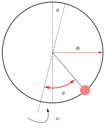
linev2 = Graphics[{Dashed, Line[{{0, 1.0}, {0, -1.0}}]}];
line2 = Graphics[Line[{{0, 0}, {0.6, -0.7}}]];
tilt = Graphics[{Dashed, Line[{{0.25, 0.97}, {-0.3, -1.2}}]}];
ar2 = Graphics[ Arrow[BezierCurve[{{-0.5, -1.3}, {-0.0, -1.55}, {-0.1, -1.1}}]]];
rAngls = {{0.7, {-11.4*Pi/8, 10.33*Pi/6}}};
directives = {Directive[Red, Thick, Arrowheads[{{-0.05, 0}, {0.05, 1}}]]};
arcsWArrows[args1 : {{_, {_, _}} ..}, dir_List: {Directive[GrayLevel[.3], Arrowheads[{{-0.05, 0}, {0.05, 1}}]]}] :=
ParametricPlot[
Evaluate[#[[1]]*{Cos[Rescale[u, {0, 2 Pi}, Abs@#[[2]]]],
Sin[Rescale[u, {0, 2 Pi}, Abs@#[[2]]]]} & /@ args1], {u, 0, 2 Pi}, PlotStyle -> dir, Axes -> False, PlotRangePadding -> .2, ImageSize -> 200] /. Line[x_, ___] :> Arrow[x]
ar3 = arcsWArrows[rAngls, {directives[[1]]}];
text1 = Graphics[ Text[Style["\[Theta]", FontSize -> 14, Purple], {0.21, -0.80}]];
text2 = Graphics[ Text[Style["\[Omega]", FontSize -> 14, Purple], {0.1, -1.3}]];
text4 = Graphics[ Text[Style["\[Alpha]", FontSize -> 14, Black], {0.1, 0.85}]];
Show[circle, arrow, ar2, line2, linev2, disk2, text1, text2, text3, text4, tilt, ar3]
 |
 |
The kinetic energy reads
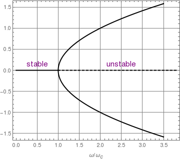
curve1 = Plot[Sqrt[x - 1], {x, 1, 3.5}, PlotStyle -> {Thick, Black}];
curve2 = Plot[-Sqrt[x - 1], {x, 1, 3.5}, PlotStyle -> {Thick, Black}];
line2 = Graphics[{Thick, Dashed, Line[{{3.8, 0}, {1, 0}}]}];
text1 = Graphics[ Text[Style["stable", FontSize -> 14, Purple], {0.5, 0.1}]];
text2 = Graphics[ Text[Style["unstable", FontSize -> 14, Purple], {2.5, 0.1}]];
Show[text1, text2, line, line2, curve1, curve2, FrameLabel -> {"\[Omega]/\!\(\*SubscriptBox[\(\[Omega]\), \(c\)]\)", None}, Frame -> True, GridLines -> Automatic]
Example:
Example: Move to chapter 4, application4 Consider the Lane--Emden type equation with an exponential nonlinearity of the solution with respect to the variable base
Example: Consider the initial value problem for undamped Duffing equation:
- Raviola, Lisandro A., Veliz, Maximiliano E., Salomone, Horacio D., Olivieri, Nestor A., and Rodriguez, Eduardo E. The bead on a rotating hoop revisited: an unexpected resonance, European Journal of Physics, 38, 2017, 015005 (13pp).
- Halloun I.A. and Hestenes D., Common sense concepts about motion, American Journal of Physics, 53, 1985, 1056
- Perez F., Granger B.E., and Hunter J.D., Python: an ecosystem for scientific computing, Computing in Science & Engineering, Volume: 13, Issue: 2, 2011, pages: 13--21. doi: 10.1109/MCSE.2010.119
- Sivardiere J., A simple mechanical model exhibiting a spontaneous symmetry breaking, American Journal of Physics, 51, 1983, 1016 https://doi.org/10.1119/1.13362
- Drugowich de Felicio J.R. and Hipolito O., Spontaneous symmetry breaking, American Journal of Physics, 53, 1985, 690
- Ochoa F. and Clavijo J., Bead, hoop, and spring as a classical spontaneous symmetr breaking problem, European Journal of Physics, 27, 2006, 1277
- Rousseaux G., Bead, hoop, and spring ...: some theoretical remarks, European Journal of Physics, 28, 2007, L7--9
- Mancuso R.V., A working mechanical model for first- and second-order phase transition and the cusp catastrope, American Journal of Physics, 68, 2000, 271
- Cross R., Coulomb's law for tolling friction, American Journal of Physics, 84, 2016, 221
Return to Mathematica page
Return to the main page (APMA0330)
Return to the Part 1 (Plotting)
Return to the Part 2 (First Order ODEs)
Return to the Part 3 (Numerical Methods)
Return to the Part 4 (Second and Higher Order ODEs)
Return to the Part 5 (Series and Recurrences)
Return to the Part 6 (Laplace Transform)
Return to the Part 7 (Boundary Value Problems)