Return to computing page for the second course APMA0340
Return to Mathematica tutorial for the second course APMA0340
Return to the main page for the course APMA0330
Return to the main page for the course APMA0340
Return to Part IV of the course APMA0330
Glossary
Spring Problems
Sometimes it is necessary to consider the second derivative when constructing a mathematical model. There are known two famous areas of applications: mechanical and electrical oscillations. For example, the motion of a mass on a vibrating spring, the torsional oscillations of a shaft with a flywheel, the flow of electric current in a simple series circuit, and many other physical problems are all described by the solution of an initial value problem of the form
Vertical spring oscillations
A spring is an object that can be deformed by a force and then return to its original shape after the force is removed. Springs come in a huge variety of different forms, but what they all share is the elasticity. This term represents the reaction of a spring (or any other object) on axial load. When a force is placed on a material, the material stretches or compresses in response to the force. When the force is removed, the matrial returns to its original form.
When studying springs and elastic deformations, the 17ᵗʰ century British physicist Robert Hooke noticed that the stress vs strain curve for many materials has a linear region. Such proportionally of the extension of the spring to the applied force is known now as Hooke's law. Robert Hooke (1635--1703) was a scientist with wide-ranging interests. He published the book Micrographia in 1665 where he first formulated the law named after him.
Consider a mass m hanging at rest on the end of a vertical spring of original length \( \ell . \) The mass causes an elongation L of the spring in the downward direction, which we assume positive. In this static situation there are two forced acting at the point where the mass is attached to the spring. The gravitational force, or weight of the mass, acts downward and has magnitude mg, where g is the acceleration due to gravity. There is also a force, which we denote as F, due to the spring that acts upward. If we assume that the elongation L of the spring is small, the spring force is very nearly proportional to L: \( F = -k\,L , \) where k is called the spring constant. Since the mass is in equilibruim, the two forces balance each other, which means that
- The weight w = mg of the mass always acrs downward.
- The spring force Fs is assumed to be proportional to the total elongation L+x of the spring and always acts to restore the spring to its natural position. If L+x is positive, then the spring is extended, and the spring force is directed upward. In theis case
\[ F_s = -k \left( L+x \right) . \]On the otehr hand, if L+x is negative, then the spring is compressed a distance |L+x|, and the spring force, which is now directed downward, is given by \( F_s = k\left\vert L+x \right\vert = -k \left( x+L \right) . \)
- The damping or resistive force Fr always acts in the direction opposite to the direction of motion of the mass. This force may be caused by different sources: internal dissipation due to compression or extension of the spring, resistance from the air or other medium, friction between the mass and the guides that constrain its motion in one dimension, or a mechanical device that imparts a resistive force to the mass. We assume that the resulting resistive force is proportional to the speed, which is usually is referred to as viscous damping:
\[ F_r = -\gamma \,\dot{x} , \]where γ is a positive constant of proportionality known as the damping constant.
Usually, a damping force is difficult to model---we discuss this issue in section devoted to pendulum motion. We benefit from this simple resistive force formula because the resulting differential equation becomes linear.
- An applied external force F(t) could be either positive or negative depending in what direction it acts and at what time. Often the external force is periodic.

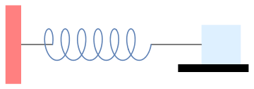
Horizontal spring oscillations
Suppose that we have a mass lying on a flat, frictionless surface and that this mass is attached to one end of a spring with the other end of the spring attached to a wall. We denote the spring displacement by x. If x>0, then the spring is stretched. If x<0, the spring is compressed. If x = 0, then the spring is in a state of equilibrium. If we pull on the mass, then the mass will oscillate back and forth across the table.
wall = Graphics[{Pink, Polygon[{{-5, -5}, {-5, 5}, {-3, 5}, {-3, -5}}]}]
line1 = Graphics[Line[{{-3, 0}, {1, 0}}]]
line2 = Graphics[Line[{{4*Pi + 1, 0}, {20, 0}}]]
box = Graphics[{LightBlue, Polygon[{{20, -2.5}, {20, 2.5}, {25, 2.5}, {25, -2.5}}]}]
ground = Graphics[ Polygon[{{17, -2.5}, {26, -2.5}, {26, -3.5}, {17, -3.5}}]]
Show[box, line1, line2, wall, spring1, ground]
By Newton's second law of motion, the force on the mass m must be
Now let us add a damping force to our system. For example, we might add a dashpot, a mechanical device that resists motion, to our system. Think of a dashpot as the small cylinder that keeps your screen door from slamming shut. The simplest assumption would be to take the damping force of the dashpot to be proportional to the velocity of the mass, \( \dot{x}(t) . \) Thus, we have will have an additional force, \( F(x) = -b\,\dot{x}(t) , \) acting on our mass, where b > 0. Our new equation for the spring-mass system is
{x'[t] == v[t], v'[t] == -(b / m) * v[t] - (k / m) * x[t], x[0] == x0, v[0] == v0}
1.4.9. Applications
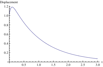
Example 4.9.2: Pure oscillations give the solutions of the following differential equation subject to the given initial conditions (displacement is 1, but velocity is zero):
soln = DSolve[{x''[t] + 25 x[t] == 0, x[0] == 1, x'[0] == 0}, x[t], t]
Plot[x[t] /. soln, {t, -1, 2.5}]
s[t_] = x[t]/.soln[[1]]
Plot[s[t],{t,0,3},AxesLabel->{"t","Displacement"}]
Example 4.9.3: Consider the initial value problem
s1[t_] = x[t] /. soln[[1]]
When does the maximum excursion occur?
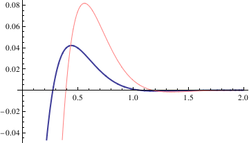
Example 4.9.4: Now we turn to a differential equation whose characteristic polynomial has a double root:
s2[t_] = x[t] /. soln[[1]]
Plot[s2[t], {t, 0.2, 3}, PlotStyle->{Thick,Magenta}]
Out[12]= E^(-3 t) (-1 + 2 t)
Out[13]=
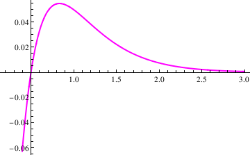
When does the extreme occur?
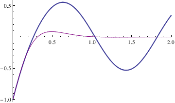
Example 4.9.5: We consider another initial value problem
x'[0] == 5}, x[t], t]
soln = DSolve[{x''[t] + 2 x'[t] + 37 x[t] == 0, x[0] == -1, x'[0] == 5}, x[t], t]
s3[t_] = x[t] /. soln[[1]]
Plot[s3[t], {t, 0, 3}, PlotRange -> {-1, 1}]
Out[20]= -(1/3) E^-t (3 Cos[6 t] - 2 Sin[6 t])
Out[21]=
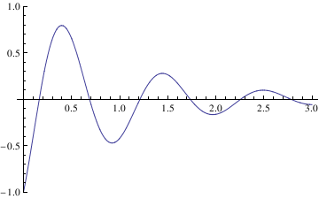
Now we define the amplitude of these oscillations:
Example 4.9.6: Forced oscillations are modeled by the following nonhomogeneous equation:
1/712 E^(-5 t) (-392 Cos[4 t] - 445 E^(5 t) Cos[4 t] +
125 E^(5 t) Cos[4 t] Cos[8 t] + 200 Sin[4 t] -
200 E^(5 t) Cos[8 t] Sin[4 t] + 200 E^(5 t) Cos[4 t] Sin[8 t] +
125 E^(5 t) Sin[4 t] Sin[8 t])}}
We extract the transient solution and the steady-state solution. First, we define the solution function:
40 E^(5 t) Cos[8 t] Sin[4 t] + 40 E^(5 t) Cos[4 t] Sin[8 t] + 25 E^(5 t) Sin[4 t] Sin[8 t])
40 Cos[8 t] Sin[4 t] - 40 Cos[4 t] Sin[8 t] - 25 Sin[4 t] Sin[8 t])}}
40 Cos[8 t] Sin[4 t] - 40 Cos[4 t] Sin[8 t] - 25 Sin[4 t] Sin[8 t])
Now we consider a similar problem but with another input function:
L[t_,x_] = x''[t] + 10 x'[t] + 41 x[t];
solnRule = DSolve[{L[t, x] == 8 *Exp[-5*t] Cos[2 t], x[0] == -1, x'[0] == 5}, x[t], t]
1/6 E^(-5 t) (-13 Cos[4 t] + 6 Cos[t]^2 Cos[4 t] +
Cos[4 t] Cos[6 t] + 3 Sin[2 t] Sin[4 t] + Sin[4 t] Sin[6 t])}}
Cos[4 t] Cos[6 t] + 3 Sin[2 t] Sin[4 t] + Sin[4 t] Sin[6 t])
E^(-5 t) C[2] Cos[4 t] + E^(-5 t) C[1] Sin[4 t] +
1/6 E^(-5 t) (6 Cos[t]^2 Cos[4 t] + Cos[4 t] Cos[6 t] +
3 Sin[2 t] Sin[4 t] + Sin[4 t] Sin[6 t])}}
1/6 E^(-5 t) (6 Cos[t]^2 Cos[4 t] + Cos[4 t] Cos[6 t] +
3 Sin[2 t] Sin[4 t] + Sin[4 t] Sin[6 t])
and the transient solution becomes
We also plot two solutions
Transient solutions could be plotted in a similar way.
Example 4.9.7: Undamped Spring with External Forcing.
Enter the coefficients and the differential equation:
ode = y''[t] + k^2*y[t] == F0*Cos[omega*t];
1/210 (-10 Cos[5 t] + 7 Cos[3 t] Cos[5 t] + 3 Cos[5 t] Cos[7 t] +
7 Sin[3 t] Sin[5 t] + 3 Sin[5 t] Sin[7 t])}}
7 Sin[3 t] Sin[5 t] + 3 Sin[5 t] Sin[7 t])
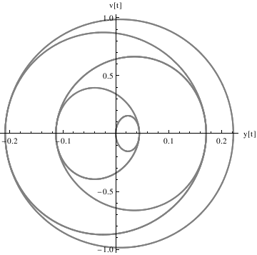
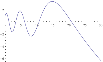
Example 4.9.8: Beats
We reconsider Example 1.4.7 for periodic input, when resonance is observed.
Enter the coefficients and the differential equation.
ode = y''[t] + k^2*y[t] == F0*Cos[omega*t];
1/90 (-10 Cos[5 t] + 9 Cos[t] Cos[5 t] + Cos[5 t] Cos[9 t] +
9 Sin[t] Sin[5 t] + Sin[5 t] Sin[9 t])}}
9 Sin[t] Sin[5 t] + Sin[5 t] Sin[9 t])
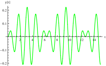
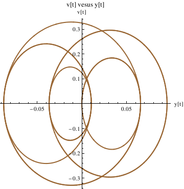
Define the derivative function as v[t], and plot the trajectory in the phase plane:
4 Cos[9 t] Sin[5 t] - 4 Cos[5 t] Sin[9 t])
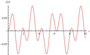
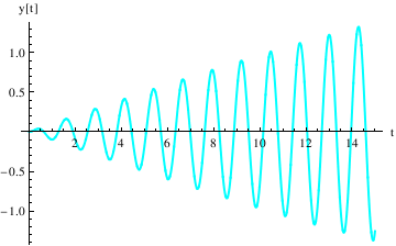
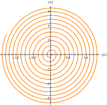
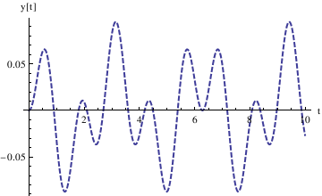
Example 4.9.9: Resonance
We repeat the commands (after quitting the kernel) here for defining the coefficients and the differential equation---now with \[omega] very close to k:
ode = y''[t] + k^2*y[t] == F0*Cos[omega*t];
DSolve[{ode, y[0] == 0, y'[0] == 0}, y[t], t]
0.010101 Cos[5. t] Cos[9.9 t] + 1. Sin[0.1 t] Sin[5. t] +
0.010101 Sin[5. t] Sin[9.9 t] }}
1.0101 Cos[4.9 t] Sin[5. t]^2
4.94949 Sin[4.9 t] Sin[5. t]^2
ode = y''[t] + k^2*y[t] == F0*Cos[omega*t];
DSolve[{ode, y[0] == 0, y'[0] == 0}, y[t], t]
y[t_] = y[t] /. %[[1]]
1/210 (-10 Cos[5 t] + 7 Cos[3 t] Cos[5 t] + 3 Cos[5 t] Cos[7 t] +
7 Sin[3 t] Sin[5 t] + 3 Sin[5 t] Sin[7 t])}}
Out[4]= 1/210 (-10 Cos[5 t] + 7 Cos[3 t] Cos[5 t] + 3 Cos[5 t] Cos[7 t] +
7 Sin[3 t] Sin[5 t] + 3 Sin[5 t] Sin[7 t])
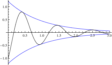
II. Aging Spring Equation
Consider the following spring equation with aging:
We solve it and plot in the following sequence of steps.
x, t] // InputForm
{{x -> Function[{t}, (BesselJ[0, 16*Sqrt[E^(-t/4)]]*
BesselY[0, 16] - BesselJ[0, 16]*BesselY[0,
16*Sqrt[E^(-t/4)]] + BesselJ[1, 16]*
BesselY[0, 16*Sqrt[E^(-t/4)]] -
BesselJ[0, 16*Sqrt[E^(-t/4)]]*BesselY[1, 16])/
(BesselJ[1, 16]*BesselY[0, 16] - BesselJ[0, 16]*
BesselY[1, 16])]}}
x, t]) // InputForm
f[t_] = x[t] /. sol[[1]]
f[0.5]
Another way to remove curly brackets:
(BesselJ[0, 16 Sqrt[E^(-t/4)]] BesselY[0, 16] -
BesselJ[0, 16] BesselY[0, 16 Sqrt[E^(-t/4)]] +
BesselJ[1, 16] BesselY[0, 16 Sqrt[E^(-t/4)]] -
BesselJ[0, 16 Sqrt[E^(-t/4)]] BesselY[1, 16])/(BesselJ[1,
16] BesselY[0, 16] - BesselJ[0, 16] BesselY[1, 16])
Return to Mathematica page
Return to the main page (APMA0330)
Return to the Part 1 (Plotting)
Return to the Part 2 (First Order ODEs)
Return to the Part 3 (Numerical Methods)
Return to the Part 4 (Second and Higher Order ODEs)
Return to the Part 5 (Series and Recurrences)
Return to the Part 6 (Laplace Transform)
Return to the Part 7 (Boundary Value